本文记录了完成《CMU 10-414/714 Deep Learning System》配套 Assignments 的过程和对应笔记。共有 6 个 hw,循序渐进地从头实现了一个深度学习框架,并利用搭建 DL 中厂常见的网络模型,包括 CNN、RNN、Transformer 等。
实验环境为 Ubuntu 24 @ WSL2。
由于官方自动评分系统目前不再接受非选课学生注册,因此本代码仅保证能够通过已有测试样例。
资源存档#
源码来自官方:Assignments
所有代码均上传至 cmu10-414-assignments: cmu10-414-assignments,如官网撤包,可通过 git 回滚获取原始代码。
hw0#
第一个 homework 共需完成 7 个函数,第一个很简单,用于熟悉评测系统,直接从第二个函数开始。
parse_mnist#
这个函数签名为:parse_mnist(image_filename, label_filename),用于读取 MNIST 手写数据集。官网 对数据集格式有详细介绍,直接下拉到 FILE FORMATS FOR THE MNIST DATABASE 这部分即可。
整个数据集分为训练集和测试集,包括数字图像和标签。标签文件内前 8Byte 记录了 magic number 和 number of items,之后按照每个样本占 1Byte 的格式组织。图像文件内前 16Byte 记录了非图像数据,之后按照行优先的顺序按照每个像素占 1Byte 的格式以此排布,每个图片共有 28×28 个像素点。
具体实现中,使用 gzip 库按字节读取数据文件,注意整个数据集需要进行标准化,即将每个像素的灰度值除以 255。完整实现为:
 1
 2
 3
 4
 5
 6
 7
 8
 9
10
11
12
13
|
def parse_mnist(image_filename, label_filename):
    image_file_handle = gzip.open(image_filename, 'rb')
    label_file_handle = gzip.open(label_filename, 'rb')
    image_file_handle.read(16)
    label_file_handle.read(8)
    image_data = image_file_handle.read()
    label_data = label_file_handle.read()
    image_file_handle.close()
    label_file_handle.close()
    X = np.frombuffer(image_data, dtype=np.uint8).reshape(-1, 28*28).astype(np.float32)
    X = X / 255.0
    y = np.frombuffer(label_data, dtype=np.uint8)
    return X, y
|
softmax_loss#
这个函数签名为:softmax_loss(Z, y),需要注意的是它计算的是 softmax 损失,或者说是交叉熵损失,而不是进行 softmax 归一化。
照着公式写两行代码即可,不用再赘述:
1
2
3
|
def softmax_loss(Z, y):
    rows = np.arange(Z.shape[0])
    return -np.mean(Z[rows, y] - np.log(np.sum(np.exp(Z), axis=1)))
|
softmax_regression_epoch#
这个函数签名为:softmax_regression_epoch(X, y, theta, lr = 0.1, batch=100),要实现的是 softmax 回归一个 epoch 上的训练过程。
首先计算出总的 batch 数,并进行这么多次的循环。在每个循环内,先从 X 和 y 中取出对应样本,然后根据公式计算即可。这里涉及到将 label 转换为独热编码的一个小技巧:E_batch = np.eye(theta.shape[1])[y_batch],其它则比较简单:
 1
 2
 3
 4
 5
 6
 7
 8
 9
10
11
|
def softmax_regression_epoch(X, y, theta, lr = 0.1, batch=100):
    total_batches = (X.shape[0] + batch - 1) // batch
    for i in range(total_batches):
        X_batch = X[i*batch:(i+1)*batch]
        y_batch = y[i*batch:(i+1)*batch]
        E_batch = np.eye(theta.shape[1])[y_batch]
        logits = X_batch @ theta
        Z_batch = np.exp(logits)
        Z_batch /= np.sum(Z_batch, axis=1, keepdims=True)
        gradients = X_batch.T @ (Z_batch - E_batch) / batch
        theta -= lr * gradients
|
nn_epoch#
这个函数签名为:nn_epoch(X, y, W1, W2, lr = 0.1, batch=100),要实现一个双层感知机在一个 epoch 上的训练过程。
跟着公式写代码计算即可,需要注意的两个点:
- ReLU 激活函数可以使用 max 函数进行实现:
Z1_batch = np.maximum(X_batch @ W1, 0)
- 除以 batch_size 这一步应该提前在计算 G2 的过程,如果放在最后更新 $\theta$ 这一步,存在精度误差,不能通过测试点。
完整代码为:
 1
 2
 3
 4
 5
 6
 7
 8
 9
10
11
12
13
14
15
16
|
def nn_epoch(X, y, W1, W2, lr = 0.1, batch=100):
    total_batches = (X.shape[0] + batch - 1) // batch
    for i in range(total_batches):
        X_batch = X[i*batch:(i+1)*batch]
        y_batch = y[i*batch:(i+1)*batch]
        E_batch = np.eye(W2.shape[1])[y_batch]
        Z1_batch = np.maximum(X_batch @ W1, 0)
        G2_batch = np.exp(Z1_batch @ W2)
        G2_batch /= np.sum(G2_batch, axis=1, keepdims=True)
        G2_batch -= E_batch
        G2_batch /= batch
        G1_batch = (Z1_batch > 0) * (G2_batch @ W2.T)
        gradients_W1 = X_batch.T @ G1_batch
        gradients_W2 = Z1_batch.T @ G2_batch
        W1 -= lr * gradients_W1
        W2 -= lr * gradients_W2
|
softmax_regression_epoch_cpp#
这个函数签名为:void softmax_regression_epoch_cpp(const float *X, const unsigned char *y, float *theta, size_t m, size_t n, size_t k, float lr, size_t batch),这是一个 softmax 回归在 cpp 上的实现版本。
与 Python 自动处理数组索引越界不同,cpp 版本要分开考虑完整的 batch 和最后一轮不完整的 batch。计算 logits 时,需要使用三轮循环模拟矩阵乘法。cpp 版本的实现可以不写出 $E_y$ 矩阵,梯度计算不用使用矩阵计算,直接使用两层循环,判断 class_idx 是否为正确的 label:softmax[sample_idx * k + class_idx] -= (y[start_idx + sample_idx] == class_idx);。
完整的代码为:
 1
 2
 3
 4
 5
 6
 7
 8
 9
10
11
12
13
14
15
16
17
18
19
20
21
22
23
24
25
26
27
28
29
30
31
32
33
34
35
36
37
38
39
40
41
42
43
44
45
46
47
48
49
50
51
52
53
54
55
56
57
58
59
60
|
void softmax_regression_epoch_cpp(const float *X, const unsigned char *y,
                                  float *theta, size_t m, size_t n, size_t k,
                                  float lr, size_t batch)
{
    size_t total_batches = (m + batch - 1) / batch;

    for(size_t i = 0; i < total_batches; i++) {
        size_t start_idx = i * batch;
        size_t end_idx = std::min(start_idx + batch, m);
        size_t current_batch_size = end_idx - start_idx;

        // Allocate memory for logits and softmax
        float* logits = new float[current_batch_size * k]();
        float* softmax = new float[current_batch_size * k]();

        // Compute logits
        for(size_t sample_idx = 0; sample_idx < current_batch_size; sample_idx++) {
            for(size_t class_idx = 0; class_idx < k; class_idx++) {
                for(size_t feature_idx = 0; feature_idx < n; feature_idx++) {
                    logits[sample_idx * k + class_idx] += X[(start_idx + sample_idx) * n + feature_idx] * theta[feature_idx * k + class_idx];
                }
            }
        }

        // Compute softmax
        for(size_t sample_idx = 0; sample_idx < current_batch_size; sample_idx++) {
            float max_logit = *std::max_element(logits + sample_idx * k, logits + (sample_idx + 1) * k);
            float sum = 0;
            for(size_t class_idx = 0; class_idx < k; class_idx++) {
                softmax[sample_idx * k + class_idx] = exp(logits[sample_idx * k + class_idx] - max_logit);
                sum += softmax[sample_idx * k + class_idx];
            }
            for(size_t class_idx = 0; class_idx < k; class_idx++) {
                softmax[sample_idx * k + class_idx] /= sum;
            }
        }

        // Compute gradient
        for(size_t sample_idx = 0; sample_idx < current_batch_size; sample_idx++) {
            for(size_t class_idx = 0; class_idx < k; class_idx++) {
                softmax[sample_idx * k + class_idx] -= (y[start_idx + sample_idx] == class_idx);
            }
        }

        // Update theta
        for(size_t feature_idx = 0; feature_idx < n; feature_idx++) {
            for(size_t class_idx = 0; class_idx < k; class_idx++) {
                float gradient = 0;
                for(size_t sample_idx = 0; sample_idx < current_batch_size; sample_idx++) {
                    gradient += X[(start_idx + sample_idx) * n + feature_idx] * softmax[sample_idx * k + class_idx];
                }
                theta[feature_idx * k + class_idx] -= lr * gradient / current_batch_size;
            }
        }

        // Free allocated memory
        delete[] logits;
        delete[] softmax;
    }
}
|
hw0 小结#
hw0 理应是在 Lecture 2 课前完成的,初学者看到一堆公式应该会很懵逼,但整个 hw 比较简单,照着公式一步步走就能完成(除了双层感知机中奇怪的精度错误),主要还是用来熟悉 NumPy 和基本的 DL 模型。
hw1#
第一个 homework 共有六个小问:正向计算、反向梯度、拓扑排序反向模式自动微分、softmax 损失、双层感知机的 SGD 算法。
Implementing forward & backward computation#
前两个小问就放在一起讨论了。第一问是通过 NumPy 的 API 实现一些常用的算子,第二问则是通过第一问的算子实现常用算子的梯度实现。
需要注意的是,notebook 中强调了第一问操作的对象是 NDArray,第二问是 Tensor。前者模拟的事这些算子的低层实现,后者则是通过调用这个算子来实现梯度计算,或者说是将梯度计算封装为另一个算子,这样就可以求梯度看作一个普通运算,进而自动求出梯度的梯度。详细解释请看 Lecture 4。
- PowerScaler
这个算子作用是对张量逐元素求幂。幂指数作为不可学习的参数,在算子实例化时就固定了,因此不用考虑对幂指数的偏导数。这个很简单,应用幂函数的求导公式即可:
 1
 2
 3
 4
 5
 6
 7
 8
 9
10
11
12
|
class PowerScalar(TensorOp):
    """Op raise a tensor to an (integer) power."""

    def __init__(self, scalar: int):
        self.scalar = scalar

    def compute(self, a: NDArray) -> NDArray:
        return array_api.power(a, self.scalar)

    def gradient(self, out_grad, node):
        a = node.inputs[0]
        return self.scalar * (power_scalar(a, self.scalar-1)) * out_grad
|
- EWiseDiv
这个算子的作用是对张量逐元素求商。梯度计算很简单,即 $a/b$ 分别对 $a$ 和 $b$ 求偏导:
1
2
3
4
5
6
7
8
9
|
class EWiseDiv(TensorOp):
    """Op to element-wise divide two nodes."""

    def compute(self, a, b):
        return array_api.true_divide(a, b)

    def gradient(self, out_grad, node):
        a, b = node.inputs
        return out_grad/b , -a/b/b*out_grad
|
- DivScalar
这个算子的作用是将整个张量同除 scalar,和 PowerScalar 一样,scalar 是不要考虑梯度的:
1
2
3
4
5
6
7
8
9
|
class DivScalar(TensorOp):
    def __init__(self, scalar):
        self.scalar = scalar

    def compute(self, a):
        return array_api.true_divide(a, self.scalar)

    def gradient(self, out_grad, node):
        return out_grad/self.scalar
|
- MatMul
这个算子的作用是矩阵乘法。这是这门课程到现在第一个具有挑战性的任务。在计算梯度时,根据课程给出的方法,可以得到如下两个表达式:
1
2
|
adjoint1 = out_grad @ transpose(b)
adjoint2 = transpose(a) @ out_grad
|
但但但是,以上只是理论推导。在实际应用中,存在两个问题:1) 矩阵乘法可能是高维矩阵而非二维矩阵相乘,例如 shape 为 (2, 2, 3, 4) 和 (2, 2, 4, 5) 的两个张量相乘;2) 张量乘法过程可能存在广播的情况,这种情况下的梯度怎么处理。
第一个问题,NumPy 基本都为我们处理好了,只要两个张量的倒数两个维度符合二维矩阵乘法且其余维度(也称为批量维度)相等,或者某个批量维度为 1(会进行广播),它们就可以进行张量乘法运算。
天下没有免费的午餐,自动广播带来便利的同时,也带来了第二个问题。求出的 adjoint 或者说偏导,应该和输入参数的维度一致,但根据公式计算得到的梯度的维度和广播后的维度一样,因此要进行 reduce 操作。
以下是我不严谨且非形式化的 reduce 操作推导:假设矩阵 $A_{m\times n}$ 经过广播后是 $A_{p\times n\times n}^\prime$,实际上参与计算的就是这个 $A^\prime$。首先直接假设在计算图上用 $A^\prime$ 替代 $A$,当 $A^\prime @B$(该节点记为 $f(x_1,…)$)的某个输入节点 $x_1$ 需要计算梯度时,就会需要计算张量 $\partial f/ \partial x_1$ 和张量 $A^\prime$ 求得的偏导之间的乘积。接下来我们把 $A$ 还原,相对应的,$f(x_1, …)$ 这个节点计算梯度就要将 $p$ 维度上的偏导数全部加起来,这体现在 $A_{p\times n\times n}^\prime$ 也是将其 $p$ 维度上的元素全部加起来,得到 $A^\prime_{m\times n}$。
上面这段描述不太清晰,总而言之就是要将广播出来的维度全部 sum 掉。
NumPy 中广播新增的维度只会放在最前面,因此只需要计算出要 sum 掉维度的个数,然后取前 $n$ 个维度即可,具体见代码:
 1
 2
 3
 4
 5
 6
 7
 8
 9
10
11
|
class MatMul(TensorOp):
    def compute(self, a, b):
        return a@b

    def gradient(self, out_grad, node):
        a, b = node.inputs
        adjoint1 = out_grad @ transpose(b)
        adjoint2 = transpose(a) @ out_grad
        adjoint1 = summation(adjoint1, axes=tuple(range(len(adjoint1.shape) - len(a.shape))))
        adjoint2 = summation(adjoint2, axes=tuple(range(len(adjoint2.shape) - len(b.shape))))
        return adjoint1, adjoint2
|
- Summation
这个算子的作用是对张量的指定维度求和。设带求和的张量 $X$ 的维度为 $s_1\times s_2\times … \times s_n$,那么求和之后的维度就是移除掉 $axes$ 中指示的维度,形式化表达为:
$$
\text{SUM}(X_{s_1\times s_2\times ... \times s_n}, axes) = [\sum_{s_i \in axes} X]_{\{s_j | j\notin axes \}}
$$
假设一个输入为的 shape 为 $3\times 2\times 4 \times 5$,在第 0 和 2 的维度上做 summation,输出的 shape 为 $2\times 5$。反向传播的过程就是先把 out_grad 扩展到 $1\times 2 \times 1\times 5$,然后广播到输入的 shape。
埋个坑,这部分还没有理解,不知道怎么形式化表达求和运算与并对其求导,误打误撞以下代码通过了测试:
 1
 2
 3
 4
 5
 6
 7
 8
 9
10
11
12
13
14
15
16
|
class Summation(TensorOp):
    def __init__(self, axes: Optional[tuple] = None):
        self.axes = axes

    def compute(self, a):
        return array_api.sum(a, axis=self.axes)

    def gradient(self, out_grad, node):
        a = node.inputs[0]
        shape = list(a.shape)
        axes = self.axes
        if axes is None:
            axes = list(range(len(shape)))
        for _ in axes:
            shape[_] = 1
        return broadcast_to(reshape(out_grad, shape), a.shape)
|
- BroadcastTo
这个算子的作用是将张量广播到指定的 shape。所谓广播,就是将数据在不存在或者大小为 1 的维度上复制多份,使之与目标 shape 相匹配。
关于广播算子正向和梯度运算的分析,可查看 MatMul 算子,其对广播过程有详细讨论。本算子实现代码为:
 1
 2
 3
 4
 5
 6
 7
 8
 9
10
11
12
13
14
|
class BroadcastTo(TensorOp):
    def __init__(self, shape):
        self.shape = shape

    def compute(self, a):
        return array_api.broadcast_to(a, self.shape)

    def gradient(self, out_grad, node):
        input_shape = node.inputs[0].shape
        ret = summation(out_grad, tuple(range(len(out_grad.shape) - len(input_shape))))
        for i, dim in enumerate(input_shape):
            if dim == 1:
              ret = summation(ret, axes=(i,))
        return reshape(ret, input_shape)
|
- Reshape
这个算子的作用是将张量重整至指定 shape。反向运算则是将张量重整至输入张量的 shape。其代码实现相当简单:
1
2
3
4
5
6
7
8
9
|
class Reshape(TensorOp):
    def __init__(self, shape):
        self.shape = shape

    def compute(self, a):
        return array_api.reshape(a, self.shape)

    def gradient(self, out_grad, node):
        return reshape(out_grad, node.inputs[0].shape)
|
- Negate
这个算子作用是将整个张量取相反数,反向运算则是再取一次相反数。其代码实现为:
1
2
3
4
5
6
|
class Negate(TensorOp):
    def compute(self, a):
        return array_api.negative(a)

    def gradient(self, out_grad, node):
        return negate(out_grad)
|
- Transpose
这个算子的作用是交换指定的两个轴,如果没指定则默认为最后两个轴。注意,这个算子的行为与 np.transpose 不一致,需要调用 API 是 np.swapaxes。反向运算则是再次交换这两个轴:
 1
 2
 3
 4
 5
 6
 7
 8
 9
10
11
12
|
class Transpose(TensorOp):
    def __init__(self, axes: Optional[tuple] = None):
        self.axes = axes

    def compute(self, a):
        if self.axes is None:
            return array_api.swapaxes(a, -1, -2)
        else:
            return array_api.swapaxes(a, *self.axes)

    def gradient(self, out_grad, node):
        return transpose(out_grad, self.axes)
|
Topological sort#
这一小问要求实现拓扑排序,涉及的知识点都是数据结构的内容,包括图的拓扑排序、后序遍历和 dfs 算法。
在问题说明中明确要求使用树的后序遍历对算法图求解其拓扑序列,简单来说就是如果本节点存在未访问的子节点(inputs),则先访问子节点,否则访问本节点。所谓访问本节点,就是将其标记为已访问,并将其放入拓扑序列。
结合 dfs 算法,求拓扑序列的代码为:
 1
 2
 3
 4
 5
 6
 7
 8
 9
10
11
12
13
14
15
|
def find_topo_sort(node_list: List[Value]) -> List[Value]:
    visited = dict()
    topo_order = []
    for node in node_list:
        if not visited.get(node, False):
            topo_sort_dfs(node, visited, topo_order)
    return topo_order

def topo_sort_dfs(node, visited: dict, topo_order):
    sons = node.inputs
    for son in sons:
        if not visited.get(son, False):
            topo_sort_dfs(son, visited, topo_order)
    visited[node] = True
    topo_order.append(node)
|
Implementing reverse mode differentiation#
终于开始组装我们的自动微分算法了!核心就是理论课中介绍的反向模式 AD 的算法为代码:

其中有几个注意点:
autograd.py 文件最后一部分提供了一个助手函数 sum_node_list(node_list),用于在不创造冗余节点的情况下,对一系列 node 求和,对应伪代码中对 $\overline{v_i}$ 求和的部分;- 只有存在输入的节点才要计算梯度,初始 input 节点是没法计算梯度的,要进行判断;
node.op.gradient 返回值类型为 Tuple | Tensor,要分类处理。node.op.gradient_as_tuple 辅助函数可确保返回类型为 tuple。
在写代码之前,最好复习一遍理论;在 debug 的过程中,可以自己画一下计算图,会有奇效。反向模式 AD 具体实现为:
 1
 2
 3
 4
 5
 6
 7
 8
 9
10
11
12
|
def compute_gradient_of_variables(output_tensor, out_grad) -> None:
    for node in reverse_topo_order:
        node.grad = sum_node_list(node_to_output_grads_list[node])
        if len(node.inputs) > 0:
            gradient = node.op.gradient(node.grad, node)
            if isinstance(gradient, tuple):
                for i, son_node in enumerate(node.inputs):
                    node_to_output_grads_list.setdefault(son_node, [])
                    node_to_output_grads_list[son_node].append(gradient[i])
            else:
                node_to_output_grads_list.setdefault(node.inputs[0], [])
                node_to_output_grads_list[node.inputs[0]].append(gradient)
|
Softmax loss#
本问题先要完成对数函数和指数函数的前向和反向计算,然后再完成 softmax 损失,也就是交叉熵损失函数。
根据说明,这里传入的 y 已经转为了独热编码。具体实现根据说明中的公式一点点写即可,没有要特别说明的:
1
2
3
4
5
6
|
def softmax_loss(Z, y_one_hot):
    batch_size = Z.shape[0]
    lhs = ndl.log(ndl.exp(Z).sum(axes=(1, )))
    rhs = (Z * y_one_hot).sum(axes=(1, ))
    loss = (lhs - rhs).sum()
    return loss / batch_size
|
SGD for a two-layer neural network#
最后一问,利用前面的组件,实现一个双层感知机及其随机梯度下降算法。注意事项:
- 这里传入的 y 的值是其 label,需要转为独热编码;
- 一定要仔细看题!在计算两个权重的更新值时,应该使用 NumPy 计算,再转为 Tensor。如果直接使用 Tensor 算子计算,每次更新都会在计算图上新增好几个节点,并指数级增长,这会导致后面一些要 600 多 batch 的测试点要跑十几分钟,实际上只要几秒钟就能跑完。如果你遇到了同样的问题,请再读一遍题目要求。
代码为:
 1
 2
 3
 4
 5
 6
 7
 8
 9
10
11
12
13
14
15
16
17
18
19
20
21
22
|
def nn_epoch(X, y, W1, W2, lr=0.1, batch=100):
    batch_cnt = (X.shape[0] + batch - 1) // batch
    num_classes = W2.shape[1]
    one_hot_y = np.eye(num_classes)[y]
    for batch_idx in range(batch_cnt):
        start_idx = batch_idx * batch
        end_idx = min(X.shape[0], (batch_idx+1)*batch)
        X_batch = X[start_idx:end_idx, :]
        y_batch = one_hot_y[start_idx:end_idx]
        X_tensor = ndl.Tensor(X_batch)
        y_tensor = ndl.Tensor(y_batch)
        first_logits = X_tensor @ W1 # type: ndl.Tensor
        first_output = ndl.relu(first_logits) # type: ndl.Tensor
        second_logits = first_output @ W2 # type: ndl.Tensor
        loss_err = softmax_loss(second_logits, y_tensor) # type: ndl.Tensor
        loss_err.backward()

        new_W1 = ndl.Tensor(W1.numpy() - lr * W1.grad.numpy())
        new_W2 = ndl.Tensor(W2.numpy() - lr * W2.grad.numpy())
        W1, W2 = new_W1, new_W2

    return W1, W2
|
hw 1 小结#
明显感觉到,这个 hw 的强度上来了。由于不太熟悉 NumPy 的运算,中间查了不少资料和别人的实现。感谢 @# xx要努力 的文章 ,不少都是参考他的实现。
最后双层感知机的调试,由于使用了 Tensor 算子来实现,跑了十几分钟,最后才发现题干已经要求使用 NumPy 运算。长了个很大的教训,下次一定好好读题。
hw2#
Q1: Weight Initialization#
Q1 实现的是几种不同的生成参数初始值的方法,结合 init_basic.py 中的辅助函数,照抄 notebook 中给的公式实现,比较简单。注意把 kwargs 传递给辅助函数,里面有 dtype、device 等信息。
 1
 2
 3
 4
 5
 6
 7
 8
 9
10
11
12
13
14
15
16
17
18
19
20
21
22
23
24
25
26
27
28
29
30
31
32
|
def xavier_uniform(fan_in, fan_out, gain=1.0, **kwargs):
    ### BEGIN YOUR SOLUTION
    a = gain * math.sqrt(6 / (fan_in + fan_out))
    return rand(fan_in, fan_out, low=-a, high=a, **kwargs)
    ### END YOUR SOLUTION


def xavier_normal(fan_in, fan_out, gain=1.0, **kwargs):
    ### BEGIN YOUR SOLUTION
    std = gain * math.sqrt(2 / (fan_in + fan_out))
    return randn(fan_in, fan_out, mean=0, std=std, **kwargs)
    ### END YOUR SOLUTION


def kaiming_uniform(fan_in, fan_out, nonlinearity="relu", **kwargs):
    assert nonlinearity == "relu", "Only relu supported currently"
    if nonlinearity == "relu":
        gain = math.sqrt(2)
    ### BEGIN YOUR SOLUTION
    bound = gain * math.sqrt(3 / fan_in)
    return rand(fan_in, fan_out, low=-bound, high=bound, **kwargs)
    ### END YOUR SOLUTION


def kaiming_normal(fan_in, fan_out, nonlinearity="relu", **kwargs):
    assert nonlinearity == "relu", "Only relu supported currently"
    if nonlinearity == "relu":
        gain = math.sqrt(2)
    ### BEGIN YOUR SOLUTION
    std = gain / math.sqrt(fan_in)
    return randn(fan_in, fan_out, mean=0, std=std, **kwargs)
    ### END YOUR SOLUTION
|
Q2: nn_basic#
在 Q2,我们将实现几个最基本的 Module 组件。在 Debug 过程中,我遇到了两个很奇怪问题:
- 所有输入和参数都是
float32 类型,但有一个输出是 float64 类型,导致过不了测试点
- 反向传播中,有一个 node 接收到的
out_grad 的 shape 比该节点的输入的 shape 大,但理论上来说二者应该是一致的
经过漫长的调试追踪,发现第一个问题是因为在实现 DivScalar 即除法时,如果输入是一个实数而非一个矩阵,numpy 进行除法运算的结果默认为 float64,解决方案是显式调用 np.true_divide 进行除法运算,并使用关键字 dtype='float32' 指定返回值类型。
第二个问题是因为 numpy 中许多运算都会进行自动广播,但是该广播操作对我们的 needle 库是不可见的,也无法添加到计算图中,因此导致了反向传播过程的 shape 不匹配。解决方案是修改修改 Q1 中基础算子的实现,在计算前检查 shape 是否匹配。修改后的 ops_mathematic.py 文件内容为:
  1
  2
  3
  4
  5
  6
  7
  8
  9
 10
 11
 12
 13
 14
 15
 16
 17
 18
 19
 20
 21
 22
 23
 24
 25
 26
 27
 28
 29
 30
 31
 32
 33
 34
 35
 36
 37
 38
 39
 40
 41
 42
 43
 44
 45
 46
 47
 48
 49
 50
 51
 52
 53
 54
 55
 56
 57
 58
 59
 60
 61
 62
 63
 64
 65
 66
 67
 68
 69
 70
 71
 72
 73
 74
 75
 76
 77
 78
 79
 80
 81
 82
 83
 84
 85
 86
 87
 88
 89
 90
 91
 92
 93
 94
 95
 96
 97
 98
 99
100
101
102
103
104
105
106
107
108
109
110
111
112
113
114
115
116
117
118
119
120
121
122
123
124
125
126
127
128
129
130
131
132
133
134
135
136
137
138
139
140
141
142
143
144
145
146
147
148
149
150
151
152
153
154
155
156
157
158
159
160
161
162
163
164
165
166
167
168
169
170
171
172
173
174
175
176
177
178
179
180
181
182
183
184
185
186
187
188
189
190
191
192
193
194
195
196
197
198
199
200
201
202
203
204
205
206
207
208
209
210
211
212
213
214
215
216
217
218
219
220
221
222
223
224
225
226
227
228
229
230
231
232
233
234
235
236
237
238
239
240
241
242
243
244
245
246
247
248
249
250
251
252
253
254
255
256
257
258
259
260
261
262
263
264
265
266
267
268
269
270
271
272
273
274
275
276
277
278
279
280
281
282
283
284
285
286
287
288
289
290
291
292
293
294
295
296
297
298
299
300
301
302
303
304
305
306
307
308
309
310
311
312
313
314
315
316
317
318
319
320
321
322
323
324
325
326
327
328
329
330
331
332
333
334
335
336
337
338
339
340
341
342
343
344
|
"""Operator implementations."""

from numbers import Number
from typing import Optional, List, Tuple, Union

from ..autograd import NDArray
from ..autograd import Op, Tensor, Value, TensorOp
from ..autograd import TensorTuple, TensorTupleOp
import numpy

# NOTE: we will import numpy as the array_api
# as the backend for our computations, this line will change in later homeworks

import numpy as array_api


class EWiseAdd(TensorOp):
    def compute(self, a: NDArray, b: NDArray):
        assert a.shape == b.shape , "The shape of lhs {} and rhs {} should be the same".format(a.shape, b.shape)
        return a + b

    def gradient(self, out_grad: Tensor, node: Tensor):
        return out_grad, out_grad


def add(a, b):
    return EWiseAdd()(a, b)


class AddScalar(TensorOp):
    def __init__(self, scalar):
        self.scalar = scalar

    def compute(self, a: NDArray):
        return a + self.scalar

    def gradient(self, out_grad: Tensor, node: Tensor):
        return out_grad


def add_scalar(a, scalar):
    return AddScalar(scalar)(a)


class EWiseMul(TensorOp):
    def compute(self, a: NDArray, b: NDArray):
        assert a.shape == b.shape, "The shape of two tensors should be the same"
        return a * b

    def gradient(self, out_grad: Tensor, node: Tensor):
        lhs, rhs = node.inputs
        return out_grad * rhs, out_grad * lhs


def multiply(a, b):
    return EWiseMul()(a, b)


class MulScalar(TensorOp):
    def __init__(self, scalar):
        self.scalar = scalar

    def compute(self, a: NDArray):
        return a * self.scalar

    def gradient(self, out_grad: Tensor, node: Tensor):
        return (out_grad * self.scalar,)


def mul_scalar(a, scalar):
    return MulScalar(scalar)(a)


class PowerScalar(TensorOp):
    """Op raise a tensor to an (integer) power."""

    def __init__(self, scalar: int):
        self.scalar = scalar

    def compute(self, a: NDArray) -> NDArray:
        ### BEGIN YOUR SOLUTION
        return array_api.power(a, self.scalar, dtype=a.dtype)
        ### END YOUR SOLUTION

    def gradient(self, out_grad, node):
        ### BEGIN YOUR SOLUTION
        a = node.inputs[0]
        return self.scalar * (power_scalar(a, self.scalar-1)) * out_grad
        ### END YOUR SOLUTION


def power_scalar(a, scalar):
    return PowerScalar(scalar)(a)


class EWisePow(TensorOp):
    """Op to element-wise raise a tensor to a power."""

    def compute(self, a: NDArray, b: NDArray) -> NDArray:
        assert a.shape == b.shape, "The shape of two tensors should be the same"
        return a**b

    def gradient(self, out_grad, node):
        if not isinstance(node.inputs[0], NDArray) or not isinstance(
            node.inputs[1], NDArray
        ):
            raise ValueError("Both inputs must be tensors (NDArray).")

        a, b = node.inputs[0], node.inputs[1]
        grad_a = out_grad * b * (a ** (b - 1))
        grad_b = out_grad * (a**b) * array_api.log(a.data)
        return grad_a, grad_b

def power(a, b):
    return EWisePow()(a, b)


class EWiseDiv(TensorOp):
    """Op to element-wise divide two nodes."""

    def compute(self, a, b):
        ### BEGIN YOUR SOLUTION
        assert a.shape == b.shape, "The shape of two tensors should be the same"
        return array_api.true_divide(a, b)
        ### END YOUR SOLUTION

    def gradient(self, out_grad, node):
        ### BEGIN YOUR SOLUTION
        a, b = node.inputs
        return out_grad/b , -a/b/b*out_grad
        ### END YOUR SOLUTION


def divide(a, b):
    return EWiseDiv()(a, b)


class DivScalar(TensorOp):
    def __init__(self, scalar):
        self.scalar = scalar

    def compute(self, a):
        ### BEGIN YOUR SOLUTION
        return array_api.true_divide(a, self.scalar, dtype=a.dtype)
        ### END YOUR SOLUTION

    def gradient(self, out_grad, node):
        ### BEGIN YOUR SOLUTION
        return out_grad/self.scalar
        ### END YOUR SOLUTION


def divide_scalar(a, scalar):
    return DivScalar(scalar)(a)


class Transpose(TensorOp):
    def __init__(self, axes: Optional[tuple] = None):
        self.axes = axes

    def compute(self, a):
        ### BEGIN YOUR SOLUTION
        if self.axes is None:
            return array_api.swapaxes(a, -1, -2)
        else:
            return array_api.swapaxes(a, *self.axes)
        ### END YOUR SOLUTION

    def gradient(self, out_grad, node):
        ### BEGIN YOUR SOLUTION
        return transpose(out_grad, self.axes)
        ### END YOUR SOLUTION


def transpose(a, axes=None):
    return Transpose(axes)(a)


class Reshape(TensorOp):
    def __init__(self, shape):
        self.shape = shape

    def compute(self, a):
        ### BEGIN YOUR SOLUTION
        expect_size = 1
        for i in self.shape:
            expect_size *= i
        real_size = 1
        for i in a.shape:
            real_size *= i
        assert expect_size == real_size , "The reshape size is not compatible"
        return array_api.reshape(a, self.shape)
        ### END YOUR SOLUTION

    def gradient(self, out_grad, node):
        ### BEGIN YOUR SOLUTION
        return reshape(out_grad, node.inputs[0].shape)
        ### END YOUR SOLUTION


def reshape(a, shape):
    return Reshape(shape)(a)


class BroadcastTo(TensorOp):
    def __init__(self, shape):
        self.shape = shape

    def compute(self, a):
        ### BEGIN YOUR SOLUTION
        assert len(self.shape) >= len(a.shape), \
            "The target shape's dimension count {} should be greater than \
                or equal to the input shape's dimension count {}".format(len(self.shape), len(a.shape))
        for i in range(len(a.shape)):
            assert a.shape[-1 - i] == self.shape[-1 - i] or a.shape[-1 - i] == 1, \
                "The input shape {} is not compatible with the target shape {}".format(a.shape, self.shape)
        return array_api.broadcast_to(a, self.shape)
        ### END YOUR SOLUTION

    def gradient(self, out_grad, node):
        ### BEGIN YOUR SOLUTION
        input_shape = node.inputs[0].shape
        ret = summation(out_grad, tuple(range(len(out_grad.shape) - len(input_shape))))
        for i in range(len(input_shape)):
            if input_shape[-1 - i] == 1 and self.shape[-1 - i] != 1:
                ret = summation(ret, (len(input_shape) - 1 - i,))
        return reshape(ret, input_shape)
        ### END YOUR SOLUTION


def broadcast_to(a, shape):
    return BroadcastTo(shape)(a)


class Summation(TensorOp):
    def __init__(self, axes: Optional[tuple] = None):
        self.axes = axes

    def compute(self, a):
        ### BEGIN YOUR SOLUTION
        return array_api.sum(a, axis=self.axes)
        ### END YOUR SOLUTION

    def gradient(self, out_grad, node):
        ### BEGIN YOUR SOLUTION
        a = node.inputs[0]
        shape = list(a.shape)
        axes = self.axes
        if axes is None:
            axes = list(range(len(shape)))
        for _ in axes:
            shape[_] = 1
        return broadcast_to(reshape(out_grad, shape), a.shape)
        ### END YOUR SOLUTION


def summation(a, axes=None):
    return Summation(axes)(a)


class MatMul(TensorOp):
    def compute(self, a, b):
        ### BEGIN YOUR SOLUTION
        return a@b
        ### END YOUR SOLUTION

    def gradient(self, out_grad, node):
        ### BEGIN YOUR SOLUTION
        a, b = node.inputs
        adjoint1 = out_grad @ transpose(b)
        adjoint2 = transpose(a) @ out_grad
        adjoint1 = summation(adjoint1, axes=tuple(range(len(adjoint1.shape) - len(a.shape))))
        adjoint2 = summation(adjoint2, axes=tuple(range(len(adjoint2.shape) - len(b.shape))))
        return adjoint1, adjoint2
        ### END YOUR SOLUTION


def matmul(a, b):
    return MatMul()(a, b)


class Negate(TensorOp):
    def compute(self, a):
        ### BEGIN YOUR SOLUTION
        return array_api.negative(a)
        ### END YOUR SOLUTION

    def gradient(self, out_grad, node):
        ### BEGIN YOUR SOLUTION
        return negate(out_grad)
        ### END YOUR SOLUTION


def negate(a):
    return Negate()(a)


class Log(TensorOp):
    def compute(self, a):
        ### BEGIN YOUR SOLUTION
        return array_api.log(a)
        ### END YOUR SOLUTION

    def gradient(self, out_grad, node):
        ### BEGIN YOUR SOLUTION
        return out_grad / node.inputs[0]
        ### END YOUR SOLUTION


def log(a):
    return Log()(a)


class Exp(TensorOp):
    def compute(self, a):
        ### BEGIN YOUR SOLUTION
        return array_api.exp(a)
        ### END YOUR SOLUTION

    def gradient(self, out_grad, node):
        ### BEGIN YOUR SOLUTION
        return out_grad * exp(node.inputs[0])
        ### END YOUR SOLUTION


def exp(a):
    return Exp()(a)


class ReLU(TensorOp):
    def compute(self, a):
        ### BEGIN YOUR SOLUTION
        return array_api.maximum(a, 0)
        ### END YOUR SOLUTION

    def gradient(self, out_grad, node):
        ### BEGIN YOUR SOLUTION
        relu_mask = Tensor(node.inputs[0].cached_data > 0)
        return out_grad * relu_mask
        ### END YOUR SOLUTION


def relu(a):
    return ReLU()(a)
|
万事俱备,接下来可以开始完成 Q2 了。
$$
Y = XW + B
$$
注意 weight 和 bias 都是 Parameter 类型,如果定义为 Tensor 类型,会导致后面实现优化器过不了测试点。该模块代码为:
 1
 2
 3
 4
 5
 6
 7
 8
 9
10
11
12
13
14
15
16
17
18
19
20
21
22
23
24
25
26
27
|
class Linear(Module):
    def __init__(
        self, in_features, out_features, bias=True, device=None, dtype="float32"
    ):
        super().__init__()
        self.in_features = in_features
        self.out_features = out_features

        ### BEGIN YOUR SOLUTION
        self.weight = init.kaiming_uniform(in_features, out_features, device=device, dtype=dtype)
        self.weight = Parameter(self.weight, device=device, dtype=dtype)
        self.bias = None
        if bias:
            self.bias = init.kaiming_uniform(out_features, 1, device=device, dtype=dtype)
            self.bias = self.bias.transpose()
            self.bias = Parameter(self.bias, device=device, dtype=dtype)
        ### END YOUR SOLUTION

    def forward(self, X: Tensor) -> Tensor:
        ### BEGIN YOUR SOLUTION
        if self.bias.shape != (1, self.out_features):
            self.bias = self.bias.reshape((1, self.out_features))
        y = ops.matmul(X, self.weight)
        if self.bias:
            y += self.bias.broadcast_to(y.shape)
        return y
        ### END YOUR SOLUTION
|
 1
 2
 3
 4
 5
 6
 7
 8
 9
10
11
12
13
|
class Sequential(Module):
    def __init__(self, *modules):
        super().__init__()
        self.modules = modules

    def forward(self, x: Tensor) -> Tensor:
        ### BEGIN YOUR SOLUTION
        y = x
        for module in self.modules:
            y = module(y)
        return y

        ### END YOUR SOLUTION
|
- LogSumExp
这里要实现的是数值稳定版本的 LogSumExp 算子。文档中直接给出了公式,这里我们给出推导过程:
$$
\begin{align*}
\log \sum_i \exp(z_i)
&= \log \sum_i \exp(z_i - \max z + \max z)\\
&=\log \sum_i[\exp(z_i - \max z) \cdot \exp(\max z)] \\
&= \log [\sum_i \exp(z_i -\max z)\cdot\exp(\max z)] \\
&=\log \sum_i \exp(z_i -\max z) + \max z
\end{align*}
$$
通过恒等变换,避免了 $\exp$ 指数运算可能导致的数值上溢的问题。
显然,数值稳定版本的梯度和原始公式的梯度一致,直接求导或者根据文章 LogSumExp梯度推导 得到其梯度计算公式为:
$$
\begin{align*}
\frac{\partial{f}}{\partial{z_j}}
&=\frac{\exp{\hat{z}_j}}{\sum_{i=1}^n\exp\hat{z}_i}\\
&=\exp(z_j - \log \sum_{i=1}^n\exp\hat{z}_i)\\
&=\exp(z_j - f)
\end{align*}
$$
惊喜地发现,LogSumExp 这个函数的梯度可以用其输入和输出来表示,那在代码实现中,只要获取该节点的输入和输出就可以计算出梯度,即:
 1
 2
 3
 4
 5
 6
 7
 8
 9
10
11
12
13
14
15
16
17
18
19
|
class LogSumExp(TensorOp):
    def __init__(self, axes: Optional[tuple] = None):
        self.axes = axes

    def compute(self, Z):
        ### BEGIN YOUR SOLUTION
        max_z = array_api.max(Z, axis=self.axes, keepdims=True)
        self.max_z = max_z
        return array_api.log(array_api.sum(array_api.exp(Z - max_z), axis=self.axes)) + max_z.squeeze()
        ### END YOUR SOLUTION

    def gradient(self, out_grad, node):
        ### BEGIN YOUR SOLUTION
        if self.axes is None:
            self.axes = tuple(range(len(node.inputs[0].shape)))
        z = node.inputs[0]
        shape = [1 if i in self.axes else z.shape[i] for i in range(len(z.shape))]
        gradient = exp(z - node.reshape(shape).broadcast_to(z.shape))
        return out_grad.reshape(shape).broadcast_to(z.shape)*gradient
|
- SoftmaxLoss
这里实现其是计算 Softmax 损失的模块,在实现过程中可以调用前面实现的数值稳定版本的 LogSumExp,其公式为:
$$
\begin{align*}
\ell_\text{softmax}(z,y) = \log \sum_{i=1}^k \exp z_i - z_y
\end{align*}
$$
代码骨架中已经提供了一个将标签转换为度和编码的辅助函数,同时记得求的损失应该是在 batch 上的均值,记得做平均。
1
2
3
4
5
6
7
8
|
class SoftmaxLoss(Module):
    def forward(self, logits: Tensor, y: Tensor):
        ### BEGIN YOUR SOLUTION
        batch_size, label_size = logits.shape
        one_hot_y = init.one_hot(label_size, y)
        true_logits = ops.summation(logits * one_hot_y, axes=(1,))
        return (ops.logsumexp(logits, axes=(1, )) - true_logits).sum()/batch_size
        ### END YOUR SOLUTION
|
- LayerNorm1d
这是第一个比较有挑战性的模块,其中涉及大量的 reshape 和广播操作,必须对每个变量的形状都了如指掌。注意,可以默认输入的 shape 为 (batch_size, feature_size)。计算公式为:
$$
\begin{align*}
y = w \circ \frac{x_i - \textbf{E}[x]}{((\textbf{Var}[x]+\epsilon)^{1/2})} + b
\end{align*}
$$
根据公式照抄即可,但是要注意中间变量的 shape:
 1
 2
 3
 4
 5
 6
 7
 8
 9
10
11
12
13
14
15
16
17
18
19
20
|
class LayerNorm1d(Module):
    def __init__(self, dim, eps=1e-5, device=None, dtype="float32"):
        super().__init__()
        self.dim = dim
        self.eps = eps
        self.weight = Parameter(init.ones(1, dim, device=device, dtype=dtype), device=device, dtype=dtype)
        ### BEGIN YOUR SOLUTION
        self.bias = Parameter(init.zeros(1, dim, device=device, dtype=dtype), device=device, dtype=dtype)
        ### END YOUR SOLUTION

    def forward(self, x: Tensor) -> Tensor:
        ### BEGIN YOUR SOLUTION
        batch_size, feature_size = x.shape
        mean = (x.sum(axes=(1, )) / feature_size).reshape((batch_size, 1)).broadcast_to(x.shape)
        var = (((x - mean) ** 2).sum(axes=(1, )) / feature_size).reshape((batch_size, 1)).broadcast_to(x.shape)
        std_x = (x - mean) / ops.power_scalar(var + self.eps, 0.5)
        weight = self.weight.broadcast_to(x.shape)
        bias = self.bias.broadcast_to(x.shape)
        return std_x * weight + bias
        ### END YOUR SOLUTION
|
- Flatten
本模块的作用是保留第一个维度为 batchsize,展平剩下维度。使用 ops.resahpe 实现即可:
1
2
3
4
5
6
7
8
9
|
class Flatten(Module):
    def forward(self, X):
        ### BEGIN YOUR SOLUTION
        assert len(X.shape) >= 2
        elem_cnt = 1
        for i in range(1, len(X.shape)):
            elem_cnt *= X.shape[i]
        return X.reshape((X.shape[0], elem_cnt))
        ### END YOUR SOLUTION
|
- BatchNorm1d
LayerNorm 是在每一个 batch 内部进行标准化操作,而 BatchNorm 是在每一个 feature 内部进行标准化操作。这就导致了每个样本都会对其他样本的推理结果产生影响,因此在推理时应动态计算均值和方差,以供推理时使用。nn.Module 中有一个 training 字段用于标识是否在训练。
与 LayerNorm 类似,在实现过程中运用了大量 reshape 和广播操作,要留意中间变量的形状。
 1
 2
 3
 4
 5
 6
 7
 8
 9
10
11
12
13
14
15
16
17
18
19
20
21
22
23
24
25
26
27
28
29
30
31
32
33
34
|
class BatchNorm1d(Module):
    def __init__(self, dim, eps=1e-5, momentum=0.1, device=None, dtype="float32"):
        super().__init__()
        self.dim = dim
        self.eps = eps
        self.momentum = momentum
        ### BEGIN YOUR SOLUTION
        self.weight = Parameter(init.ones(1, dim, device=device, dtype=dtype), device=device, dtype=dtype)
        self.bias = Parameter(init.zeros(1, dim, device=device, dtype=dtype), device=device, dtype=dtype)
        self.running_mean = init.zeros(dim, device=device, dtype=dtype)
        self.running_var = init.ones(dim, device=device, dtype=dtype)
        ### END YOUR SOLUTION

    def forward(self, x: Tensor) -> Tensor:
        ### BEGIN YOUR SOLUTION
        if self.weight.shape != (1, self.dim):
            self.weight = self.weight.reshape((1, self.dim))
        if self.bias.shape != (1, self.dim):
            self.bias = self.bias.reshape((1, self.dim))
        if self.training:
            batch_size, feature_size = x.shape
            mean = (x.sum(axes=(0, )) / batch_size).reshape((1, feature_size))
            var = (((x - mean.broadcast_to(x.shape)) ** 2).sum(axes=(0, )) / batch_size).reshape((1, feature_size))
            self.running_mean = self.running_mean *(1 - self.momentum) + mean.reshape(self.running_mean.shape) * ( self.momentum)
            self.running_var = self.running_var *(1 - self.momentum) + var.reshape(self.running_var.shape) * (self.momentum)
            mean = mean.broadcast_to(x.shape)
            var = var.broadcast_to(x.shape)
            std_x = (x - mean) / ops.power_scalar(var + self.eps, 0.5)
            weight = self.weight.broadcast_to(x.shape)
            bias = self.bias.broadcast_to(x.shape)
            return std_x * weight + bias
        else:
            std_x = (x - self.running_mean.broadcast_to(x.shape)) / ops.power_scalar(self.running_var.broadcast_to(x.shape) + self.eps, 0.5)
            return std_x * self.weight.broadcast_to(x.shape) + self.bias.broadcast_to(x.shape)
|
- Dropout
Dropout 说白了就是以概率 p 随机丢弃一部分输入,并把剩下的输入进行缩放,以确保下一层的输入期望不变。代码骨架提供了 init.randb 用于生成服从二项分布的布尔序列。代码实现为:
 1
 2
 3
 4
 5
 6
 7
 8
 9
10
11
12
|
class Dropout(Module):
    def __init__(self, p=0.5):
        super().__init__()
        self.p = p

    def forward(self, x: Tensor) -> Tensor:
        ### BEGIN YOUR SOLUTION
        if not self.training:
            return x
        mask = init.randb(*x.shape, p=1 - self.p)
        return x * mask / (1 - self.p)
        ### END YOUR SOLUTION
|
- Residual
残差模块就是将其它模块的输出和输入的和作为新的输出,实现比较简单:
1
2
3
4
5
6
7
8
9
|
class Residual(Module):
    def __init__(self, fn: Module):
        super().__init__()
        self.fn = fn

    def forward(self, x: Tensor) -> Tensor:
        ### BEGIN YOUR SOLUTION
        return x + self.fn(x)
        ### END YOUR SOLUTION
|
Q3: Optimizer Implementation#
在本问题中,我们将实现优化器模块。优化器模块的作用是根据 loss.backward() 计算出的梯度,更新模型的参数。
需要注意的是,本模块默认启用 l2 正则化或者说 weight decay,因此梯度等于 param.grad + weight_decay * param。
- SGD
首先要实现的优化器是随机梯度下降,注意在更新参数时要先使用 data 方法创建该参数的副本,以避免计算图越来越大。这里还使用了移动平均来计算梯度,初始值默认为 0。代码实现如下:
 1
 2
 3
 4
 5
 6
 7
 8
 9
10
11
12
13
14
15
16
17
|
class SGD(Optimizer):
    def __init__(self, params, lr=0.01, momentum=0.0, weight_decay=0.0):
        super().__init__(params)
        self.lr = lr
        self.momentum = momentum
        self.u = {}
        self.weight_decay = weight_decay

    def step(self):
        ### BEGIN YOUR SOLUTION
        for param in self.params:
            if param.grad is not None:
                if param not in self.u:
                    self.u[param] = ndl.zeros_like(param.grad, requires_grad=False)
                self.u[param] = self.momentum * self.u[param].data + (1 - self.momentum) * (param.grad.data + self.weight_decay * param.data)
                param.data = param.data - self.lr * self.u[param]
        ### END YOUR SOLUTION
|
 1
 2
 3
 4
 5
 6
 7
 8
 9
10
11
12
13
14
15
16
17
18
19
20
21
22
23
24
25
26
27
28
29
30
31
32
33
34
35
36
37
38
39
40
|
class Adam(Optimizer):
    def __init__(
        self,
        params,
        lr=0.01,
        beta1=0.9,
        beta2=0.999,
        eps=1e-8,
        weight_decay=0.0,
    ):
        super().__init__(params)
        self.lr = lr
        self.beta1 = beta1
        self.beta2 = beta2
        self.eps = eps
        self.weight_decay = weight_decay
        self.t = 0

        self.m = {}
        self.v = {}

    def step(self):
        ### BEGIN YOUR SOLUTION
        self.t += 1
        for param in self.params:
            if param.grad is not None:
                if param not in self.m.keys():
                    self.m[param] = ndl.zeros_like(param.grad, requires_grad=False)
                if param not in self.v.keys():
                    self.v[param] = ndl.zeros_like(param.grad, requires_grad=False)
                grad = param.grad.data + self.weight_decay * param.data
                self.m[param] = self.beta1 * self.m[param] + (1 - self.beta1) * grad.data
                self.v[param] = self.beta2 * self.v[param] + (1 - self.beta2) * grad.data * grad.data
                u_hat = self.m[param].data / (1 - self.beta1 ** self.t)
                v_hat = self.v[param].data / (1 - self.beta2 ** self.t)
                param.data = param.data - self.lr * u_hat.data / (ndl.ops.power_scalar(v_hat.data, 0.5) + self.eps).data


        ### END YOUR SOLUTION
|
Q4: DataLoader Implementation#
在本问题中,我们将实现一些数据处理、Dataset 和 DataLoader 类。Dataset 类用于提供标准接口来访问数据集,DataLoader 类是从数据集读取一个 batch 的迭代器。
- RandomFlipHorizontal
这个方法是按照概率 p 反转一张图片。注意输入数据的格式是 H*W*C,因此只要使用 np.flip 对 W 轴进行翻转即可。
 1
 2
 3
 4
 5
 6
 7
 8
 9
10
11
12
13
14
15
16
17
18
19
|
class RandomFlipHorizontal(Transform):
    def __init__(self, p = 0.5):
        self.p = p

    def __call__(self, img):
        """
        Horizonally flip an image, specified as an H x W x C NDArray.
        Args:
            img: H x W x C NDArray of an image
        Returns:
            H x W x C ndarray corresponding to image flipped with probability self.p
        Note: use the provided code to provide randomness, for easier testing
        """
        flip_img = np.random.rand() < self.p
        ### BEGIN YOUR SOLUTION
        if flip_img:
            img = np.flip(img, axis=1)
        return img
        ### END YOUR SOLUTION
|
- RandomCrop
这个方法是对原图进行随机裁剪。其实现裁剪的流程是:先在上下左右填充 padding 个空白像素,然后根据上下偏移量 shift_y 和左右偏移量 shift_y,在填充图中裁切出与原图大小相同的图片。
 1
 2
 3
 4
 5
 6
 7
 8
 9
10
11
12
13
14
15
16
17
18
19
|
class RandomCrop(Transform):
    def __init__(self, padding=3):
        self.padding = padding

    def __call__(self, img):
        """ Zero pad and then randomly crop an image.
        Args:
             img: H x W x C NDArray of an image
        Return
            H x W x C NAArray of cliped image
        Note: generate the image shifted by shift_x, shift_y specified below
        """
        shift_x, shift_y = np.random.randint(low=-self.padding, high=self.padding+1, size=2)
        ### BEGIN YOUR SOLUTION
        img_size = img.shape
        img = np.pad(img, ((self.padding, self.padding), (self.padding, self.padding), (0, 0)), 'constant')
        img = img[self.padding + shift_x:self.padding + shift_x + img_size[0], self.padding + shift_y:self.padding + shift_y + img_size[1], :]
        return img
        ### END YOUR SOLUTION
|
- MNISTDataset
这里要实现针对 MNIST 数据集的 Dataset 子类,作为其子类,要实现三个方法:__init__ 方法初始化图片、标签和数据处理函数、__len__ 返回数据集样本数、__getitem__ 方法获取指定下标的数据集。
要注意的是:1) 使用之前实现的 parse_mnist 方法来解析 MNIST 数据集;2) Dataset 父类提供了 apply_transforms 方法对图片进行处理;3) __getitem__ 方法最好支持以列表指定的多下标以批量读取数据集;4) 图片处理函数接受的数据格式是 H*W*C,但 __getitem__ 返回值的格式应当为 batch_size*n。
代码实现为:
 1
 2
 3
 4
 5
 6
 7
 8
 9
10
11
12
13
14
15
16
17
18
19
20
21
22
|
class MNISTDataset(Dataset):
    def __init__(
        self,
        image_filename: str,
        label_filename: str,
        transforms: Optional[List] = None,
    ):
        ### BEGIN YOUR SOLUTION
        self.transforms = transforms
        self.X, self.y = parse_mnist(image_filename, label_filename)

        ### END YOUR SOLUTION
    def __getitem__(self, index) -> object:
        ### BEGIN YOUR SOLUTION
        x = self.apply_transforms(self.X[index].reshape(28, 28, -1))
        return x.reshape(-1, 28*28), self.y[index]
        ### END YOUR SOLUTION

    def __len__(self) -> int:
        ### BEGIN YOUR SOLUTION
        return self.X.shape[0]
        ### END YOUR SOLUTION
|
- Dataloader
Dataloader 类是一个迭代器,也挺简单的,见码知义:
 1
 2
 3
 4
 5
 6
 7
 8
 9
10
11
12
13
14
15
16
17
18
19
20
21
22
23
24
25
26
27
28
29
30
31
32
33
34
35
36
37
38
39
40
41
42
43
44
45
46
|
class DataLoader:
    r"""
    Data loader. Combines a dataset and a sampler, and provides an iterable over
    the given dataset.
    Args:
        dataset (Dataset): dataset from which to load the data.
        batch_size (int, optional): how many samples per batch to load
            (default: ``1``).
        shuffle (bool, optional): set to ``True`` to have the data reshuffled
            at every epoch (default: ``False``).
     """
    dataset: Dataset
    batch_size: Optional[int]

    def __init__(
        self,
        dataset: Dataset,
        batch_size: Optional[int] = 1,
        shuffle: bool = False,
    ):

        self.dataset = dataset
        self.shuffle = shuffle
        self.batch_size = batch_size
        if not self.shuffle:
            self.ordering = np.array_split(np.arange(len(dataset)),
                                           range(batch_size, len(dataset), batch_size))

    def __iter__(self):
        ### BEGIN YOUR SOLUTION
        if self.shuffle:
            self.ordering = np.array_split(np.random.permutation(len(self.dataset)),
                                           range(self.batch_size, len(self.dataset), self.batch_size))
        self.index = 0
        ### END YOUR SOLUTION
        return self

    def __next__(self):
        ### BEGIN YOUR SOLUTION
        if self.index >= len(self.ordering):
            raise StopIteration
        else:
            batch = [Tensor.make_const(x) for x in self.dataset[self.ordering[self.index]]]
            self.index += 1
            return batch
        ### END YOUR SOLUTION
|
Q5: MLPResNet Implementation#
到此为止,我们的 needle 库的各基本组件都实现好了,在本问题中,我们将使用他们拼出 MLP ResNet,并在 MNIST 数据集上进行训练。
- Residual Block
首先是实现一个残差块,按照下图将这一块块积木拼出来就行:

 1
 2
 3
 4
 5
 6
 7
 8
 9
10
11
12
13
14
15
16
|
def ResidualBlock(dim, hidden_dim, norm=nn.BatchNorm1d, drop_prob=0.1):
    ### BEGIN YOUR SOLUTION
    return nn.Sequential(
        nn.Residual(
            nn.Sequential(
                nn.Linear(dim, hidden_dim),
                norm(hidden_dim),
                nn.ReLU(),
                nn.Dropout(drop_prob),
                nn.Linear(hidden_dim, dim),
                norm(dim),
            )
        ),
        nn.ReLU(),
    )
    ### END YOUR SOLUTION
|
- MLP ResNet
同样是拼积木,注意这里面有 num_blocks 个 Residual Block。

 1
 2
 3
 4
 5
 6
 7
 8
 9
10
11
12
13
14
15
16
|
def MLPResNet(
    dim,
    hidden_dim=100,
    num_blocks=3,
    num_classes=10,
    norm=nn.BatchNorm1d,
    drop_prob=0.1,
):
    ### BEGIN YOUR SOLUTION
    return nn.Sequential(
        nn.Linear(dim, hidden_dim),
        nn.ReLU(),
        *[ResidualBlock(hidden_dim, hidden_dim//2, norm, drop_prob) for _ in range(num_blocks)],
        nn.Linear(hidden_dim, num_classes),
    )
    ### END YOUR SOLUTION
|
- Epoch
Epoch 方法用来执行一个 epoch 的训练或者推理,并返回平均错误率或者平均损失,这个函数的逻辑是:实例化损失函数 - 从 DataLoader 获取输入 - 模型推理 - 计算损失 - 重置梯度 - 反向传播 - 更新参数 - 计算错误率。
 1
 2
 3
 4
 5
 6
 7
 8
 9
10
11
12
13
14
15
16
17
18
19
20
21
22
23
24
|
def epoch(dataloader, model, opt=None):
    np.random.seed(4)
    ### BEGIN YOUR SOLUTION
    loss_func = nn.SoftmaxLoss()
    error_count = 0
    loss = 0
    for x, y in dataloader:
        if opt is None:
            model.eval()
        else:
            model.train()
        y_pred = model(x)
        batch_loss = loss_func(y_pred, y)
        loss += batch_loss.numpy() * x.shape[0]
        if opt is not None:
            opt.reset_grad()
            batch_loss.backward()
            opt.step()
        y = y.numpy()
        y_pred = y_pred.numpy()
        y_pred = np.argmax(y_pred, axis=1)
        error_count += np.sum(y_pred != y)
    return error_count / len(dataloader.dataset), loss / len(dataloader.dataset)
    ### END YOUR SOLUTION
|
- Train MNIST
本方法用于在 MNIST 数据集上训练一个 MLP ResNet,本方法的逻辑是:实例化 Dataset- 实例化 DataLoader- 实例化模型 - 实例化优化器 - 迭代 epoch
 1
 2
 3
 4
 5
 6
 7
 8
 9
10
11
12
13
14
15
16
17
18
19
20
21
22
23
24
|
def train_mnist(
    batch_size=100,
    epochs=10,
    optimizer=ndl.optim.Adam,
    lr=0.001,
    weight_decay=0.001,
    hidden_dim=100,
    data_dir="data",
):
    np.random.seed(4)
    ### BEGIN YOUR SOLUTION
    train_dataset = ndl.data.MNISTDataset(data_dir+"/train-images-idx3-ubyte.gz", data_dir+"/train-labels-idx1-ubyte.gz")
    test_dataset = ndl.data.MNISTDataset(data_dir+"/t10k-images-idx3-ubyte.gz", data_dir+"/t10k-labels-idx1-ubyte.gz")
    train_dataloader = ndl.data.DataLoader(train_dataset, batch_size=batch_size, shuffle=True)
    test_dataloader = ndl.data.DataLoader(test_dataset, batch_size=batch_size)
    model = MLPResNet(784, hidden_dim)
    opt = optimizer(model.parameters(), lr=lr, weight_decay=weight_decay)
    for i in range(epochs):
        train_error, train_loss = epoch(train_dataloader, model, opt)
        test_error, test_loss = epoch(test_dataloader, model)
        # print(f"Epoch {i+1}/{epochs} Train Error: {train_error:.4f} Train Loss: {train_loss:.4f} Test Error: {test_error:.4f} Test Loss: {test_loss:.4f}")
    return train_error, train_loss, test_error, test_loss

    ### END YOUR SOLUTION
|
hw2 小结#
到这里,hw2 就已经完结啦。拖拖拖,拖了一个月才做完,本课程的 test 不是很严格,在 Debug hw2 的过程中发现了不少 hw1 中的错误。遇到问题除了自己调试,也建议参考一下别人的实现,能够提升找到问题所在的效率。
hw3#
在本次实验中,我们将构建一个简单的底层库,用于实现 NDArray。之前我们是用 NunPy 来实现,这次我们将手动实现该 CPU 和 GPU 版本的底层库,并且不调用现有的高度优化的矩阵乘法或其他操作代码。
Part 1: Python array operations#
第一个部分是通过 Python 代码修改 strides、shape、offset 字段来实现一些操作,由于不涉及底层,使用 Python 来实现这些方法效率已经够高了。
在实现前,先浏览一遍 ndarray.py,其提供大量辅助函数以简化实现过程。
- reshape
reshape 操作就是按照另一种方式来解析内存中的连续一维数据。代码骨架提供了 NDArray.as_strided 方法将一个 NDArray 转换为指定 shape 和 strides,还有 NDArray.compact_strides 方法根据 shape 生成紧密排列情况下的 strides。
使用以上辅助函数后,reshape 的实现就相当简单:
1
2
3
4
|
def reshape(self, new_shape):
		assert prod(self.shape) == prod(new_shape), "Product of shapes must be equal"
	assert self.is_compact(), "Matrix must be compact"
	return self.as_strided(new_shape, NDArray.compact_strides(new_shape))
|
- permute
permute 操作指的是对 NDArray 的轴进行重排列,例如原始轴排列的顺序是 BHWC,按照 (0,3,1,2) 方式重排列,得到的轴的顺序是 BCHW。重排后索引为 [i, j, k, l],则重排前索引为 [i, k, l, j]。假设重排前的 strides 是 m, n, p, q,那么使用重排前索引得到元素下标为 im+kn+lp+jq = im+jq+kn+lp,即重排后索引对应的 strides 是 m, q, n, p,即将原始 strides 按照指定序列重排即可得到重排后对应的 strides。
1
2
3
4
|
def permute(self, new_axes):
	new_shape = tuple(self.shape[i] for i in new_axes)
	new_strides = tuple(self.strides[i] for i in new_axes)
	return NDArray.make(shape=new_shape, strides=new_strides, device=self.device, handle=self._handle, offset=self._offset)
|
- broadcast_to
广播操作很好理解,就是将元素在某些维度上复制,例如 (1, 9, 8, 1) -> (9, 9, 8, 2),那么广播后索引为 (m, n, p, q) 在原始数组上的索引就是 (0, n, p, 0),即广播的维度上 strides 置为 0 即可实现该效果。
1
2
3
4
5
6
7
8
9
|
def broadcast_to(self, new_shape):
	assert all(
		new_shape[i] == self.shape[i] or self.shape[i] == 1
		for i in range(len(self.shape))
	), "Invalid broadcast shape"
	new_strides = tuple(
		self.strides[i] if self.shape[i] == new_shape[i] else 0 for i in range(len(self.shape))
	)
	return self.compact().as_strided(new_shape, new_strides)
|
- __getitem__
getitem 用于获取制定索引的元素,并以 NDArray 的形式返回。这里需要注意的是索引都是 slice 对象,代码已完成了对索引的预处理,保证所有的索引都是标准 slice,即其 start、stop、step 属性都存在,且在对应 shape 范围内。
结果的 shape 计算比较简单,计算每个维度上的切片包含几个元素即可。strides 用于根据索引计算索引元素在一维数组中的下标,如果该维度上切片步长不为 1,那相当于每次都要跳过几个元素来访问下个元素,定量计算不难发现,新的 strides 就等于该维度上 slice.step 乘上对应的 strides。
接下来计算 offset,由于切片中存在 start 值,因此如果待访问的索引存在某个维度上索引值小于对应切片上的 start 值的,这个元素不应存在新的 NDArray 上。例如,切片在每个维度上的 start 值为 (2, 3, 4, 5),那么原始索引 (1, 3, 4, 5) 或者 (2, 3, 4, 1) 都在切片后的首个元素之前,应该被 offset 覆盖。因此,offset 值等于每个维度上的 slice.start 乘上对应的 strides。
1
2
3
4
5
6
7
8
|
def __getitem__(self, idxs):
	...
	### BEGIN YOUR SOLUTION
	shape = tuple(max(0, (s.stop - s.start + s.step - 1) // s.step) for s in idxs)
	strides = tuple(s.step * self.strides[i] for i, s in enumerate(idxs))
	offset = reduce(operator.add, (s.start * self.strides[i] for i, s in enumerate(idxs)))
	return NDArray.make(shape, strides, device=self.device, handle=self._handle, offset=offset)
	### END YOUR SOLUTION
|
Part 2: CPU Backend - Compact and setitem#
在本部分中,我们将实现 CPU 版本的 compact 和 setitem,前者用于在内存中创建一份紧密排列的数据副本,后者用于在内存中根据给定的数据赋值。
二者有个共同点,就是涉及到可变循环展开。即,由于给定 NDArray 的维度数量是不确定的,无法通过 n 重循环对数据进行遍历。此处我采用的思路是维护一个索引 (0, 0, 0, ..., 0),每次手动在最后一位执行 +1 操作,当达到对应维度的 shape 值时则进位,直至最高位也向前进位,说明遍历完毕。
这里我定义了两个辅助函数 bool next_index(std::vector<int32_t>& index, const std::vector<int32_t>& shape) 和 size_t index_to_offset(const std::vector<int32_t>& index, const std::vector<int32_t>& strides, const size_t offset),分别用于遍历索引和将索引转换为下标。二者实现为:
 1
 2
 3
 4
 5
 6
 7
 8
 9
10
11
12
13
14
15
16
17
18
19
20
21
22
23
24
25
26
27
28
29
30
31
32
33
34
35
36
37
38
39
40
41
42
43
44
45
46
47
48
49
|
bool next_index(std::vector<int32_t>& index, const std::vector<int32_t>& shape) {
  /**
   * Increment the index by one, and return true if the index is still valid
   *
   * Args:
   *  index: current index
   *  shape: shape of the array
   *
   * Returns:
   *  true if the index is still valid, false otherwise
   */
  if(index.size() == 0){
    return false;
  }
  index[index.size()-1]++;
  for(int i=index.size()-1; i>=0; i--){
    if(index[i] >= shape[i]){
      index[i] = 0;
      if(i > 0){
        index[i-1]++;
      }
      else {
        return false;
      }
    }
    else {
      return true;
    }
  }
}

size_t index_to_offset(const std::vector<int32_t>& index, const std::vector<int32_t>& strides, const size_t offset) {
  /**
   * Convert an index to an offset
   *
   * Args:
   *  index: index to convert
   *  strides: strides of the array
   *  offset: offset of the array
   *
   * Returns:
   *  offset of the index
   */
  size_t res = offset;
  for(int i=0; i<index.size(); i++){
    res += index[i] * strides[i];
  }
  return res;
}
|
- compact
compact 函数只要在预分配内存的 out 上将每个位置的值写入即可。鉴于 out 在内存中是连续的,可以使用 out_index++ 来逐个访问,原始数据则通过上述两个辅助函数进行访问:
 1
 2
 3
 4
 5
 6
 7
 8
 9
10
|
void Compact(const AlignedArray& a, AlignedArray* out, std::vector<int32_t> shape, std::vector<int32_t> strides, size_t offset) {
  /// BEGIN SOLUTION
  auto a_index = std::vector<int32_t>(shape.size(), 0);
  for (int out_index = 0; out_index < out->size; out_index++) {
    size_t a_offset = index_to_offset(a_index, strides, offset);
    out->ptr[out_index] = a.ptr[a_offset];
    next_index(a_index, shape);
  }
  /// END SOLUTION
}
|
- setitem
setitem 按照是否为标量有两个版本,但都挺简单,利用好两个辅助函数逐个访问对应下标即可:
 1
 2
 3
 4
 5
 6
 7
 8
 9
10
11
12
13
14
15
16
17
18
19
20
21
|
void EwiseSetitem(const AlignedArray& a, AlignedArray* out, std::vector<int32_t> shape, std::vector<int32_t> strides, size_t offset) {
  /// BEGIN SOLUTION
  auto out_index = std::vector<int32_t>(shape.size(), 0);
  for (int a_index = 0; a_index < a.size; a_index++) {
    size_t out_offset = index_to_offset(out_index, strides, offset);
    out->ptr[out_offset] = a.ptr[a_index];
    next_index(out_index, shape);
  }
  /// END SOLUTION
}

void ScalarSetitem(const size_t size, scalar_t val, AlignedArray* out, std::vector<int32_t> shape, td::vector<int32_t> strides, size_t offset) {
  /// BEGIN SOLUTION
  auto out_index = std::vector<int32_t>(shape.size(), 0);
  for (int i = 0; i < size; i++) {
    size_t out_offset = index_to_offset(out_index, strides, offset);
    out->ptr[out_offset] = val;
    next_index(out_index, shape);
  }
  /// END SOLUTION
}
|
Part 3: CPU Backend - Elementwise and scalar operations#
在本 Part 中,我们将完成一些非常简单的算子的 CPU 版本,本任务主要是用于熟悉在 pybind 中注册 cpp 函数的流程。文档中提到,鼓励使用模板、宏等简化实现。
我没有为每个算子都写一个显式函数声明和定义,我首先实现了 void EwiseOp(const AlignedArray& a, const AlignedArray& b, AlignedArray* out, std::function<scalar_t(scalar_t, scalar_t)> op) 和 void ScalarOp(const AlignedArray& a, scalar_t val, AlignedArray* out, std::function<scalar_t(scalar_t, scalar_t)> op),分别用于逐元素和统一执行函数 op,通过传入不同的函数 op 可以实现不同的操作。
 1
 2
 3
 4
 5
 6
 7
 8
 9
10
11
12
13
14
15
16
17
18
19
20
21
22
23
24
25
26
27
28
29
|
void EwiseOp(const AlignedArray& a, const AlignedArray& b, AlignedArray* out, std::function<scalar_t(scalar_t, scalar_t)> op) {
  /**
   * Element-wise operation on two arrays
   *
   * Args:
   *   a: first array
   *   b: second array
   *   out: output array
   *   op: operation to perform
   */
  for (size_t i = 0; i < a.size; i++) {
    out->ptr[i] = op(a.ptr[i], b.ptr[i]);
  }
}

void ScalarOp(const AlignedArray& a, scalar_t val, AlignedArray* out, std::function<scalar_t(scalar_t, scalar_t)> op) {
  /**
   * Element-wise operation on an array and a scalar
   *
   * Args:
   *   a: array
   *   val: scalar
   *   out: output array
   *   op: operation to perform
   */
  for (size_t i = 0; i < a.size; i++) {
    out->ptr[i] = op(a.ptr[i], val);
  }
}
|
再通过 lambda 表达式对上面这两个函数部分实例化(柯里化),以便其只接受两个参数 a, b 并在 pybind 中注册。
举个栗子,如果想注册一个按元素乘法,那么完整的代码为:
1
2
3
|
m.def("ewise_mul", [](const AlignedArray& a, const AlignedArray& b, AlignedArray* out) {
    EwiseOp(a, b, out, std::multiplies<scalar_t>());
});
|
从外向内看,m.def 用于在 pybind 中注册一个方法,该方法名由第一个参数指定,即 ewise_mul,第二个参数用于指定对应的 cpp 函数,这里可以接受函数指针、匿名函数等。注意,在 python 我们调用 ewise_mul,只传入两个 NDArray,因此我们需要对接受三个参数的 EwiseOp 柯里化,即传入 std::multiplies<scalar_t>() 给 EwiseOp,并将其封装为一个匿名函数。
注册方法的这一步每次都要创建一个匿名函数,有点复杂了,这一步也能抽象为一个宏,即:
 1
 2
 3
 4
 5
 6
 7
 8
 9
10
11
12
13
14
15
|
  #define REGISTER_EWISW_OP(NAME, OP) \
    m.def(NAME, [](const AlignedArray& a, const AlignedArray& b, AlignedArray* out) { \
      EwiseOp(a, b, out, OP); \
    });

  #define REGISTER_SCALAR_OP(NAME, OP) \
    m.def(NAME, [](const AlignedArray& a, scalar_t val, AlignedArray* out) { \
      ScalarOp(a, val, out, OP); \
    });
  #define REGISTER_SINGLE_OP(NAME, OP) \
    m.def(NAME, [](const AlignedArray& a, AlignedArray* out) { \
      for (size_t i = 0; i < a.size; i++) { \
        out->ptr[i] = OP(a.ptr[i]); \
      } \
    });
|
上述三个宏,分别用于注册按元素、按标量的双目运算符,和单目运算符在 pybind 中的注册。
应用这些宏,注册所有指定的方法:
 1
 2
 3
 4
 5
 6
 7
 8
 9
10
11
12
13
14
|
  REGISTER_EWISW_OP("ewise_mul", std::multiplies<scalar_t>());
  REGISTER_SCALAR_OP("scalar_mul", std::multiplies<scalar_t>());
  REGISTER_EWISW_OP("ewise_div", std::divides<scalar_t>());
  REGISTER_SCALAR_OP("scalar_div", std::divides<scalar_t>());
  REGISTER_SCALAR_OP("scalar_power", static_cast<scalar_t(*)(scalar_t, scalar_t)>(std::pow));
  REGISTER_EWISW_OP("ewise_maximum", static_cast<scalar_t(*)(scalar_t, scalar_t)>(std::fmax));
  REGISTER_SCALAR_OP("scalar_maximum", static_cast<scalar_t(*)(scalar_t, scalar_t)>(std::fmax));
  REGISTER_EWISW_OP("ewise_eq", std::equal_to<scalar_t>());
  REGISTER_SCALAR_OP("scalar_eq", std::equal_to<scalar_t>());
  REGISTER_EWISW_OP("ewise_ge", std::greater_equal<scalar_t>());
  REGISTER_SCALAR_OP("scalar_ge", std::greater_equal<scalar_t>());
  REGISTER_SINGLE_OP("ewise_log", std::log);
  REGISTER_SINGLE_OP("ewise_exp", std::exp);
  REGISTER_SINGLE_OP("ewise_tanh", std::tanh);
|
注意,其中 std::pow 等有多个重载版本,通过 static_cast 关键字可以指定版本。
Part 4: CPU Backend - Reductions#
这里要实现两个归约算子 max 和 sum,为了简化实现,这里只对单个维度进行归约。即便在单个维度上,想要实现归约运算也是相当困难的,因此本任务还进行了简化:在调用归约算子前会将待归约维度重排到最后一个维度上,并在调用结束后自动恢复,因此我们只要实现对最后一个维度的归约运算。
经过一系列简化操作,这两个算子实现起来有点过于简单了:对连续的 reduce_size 个元素进行 max/sum 运算作为输出的新元素即可,最后记得在 pybind 中注册这两个方法:
 1
 2
 3
 4
 5
 6
 7
 8
 9
10
11
12
13
14
15
16
17
18
19
20
21
|
void ReduceMax(const AlignedArray& a, AlignedArray* out, size_t reduce_size) {
  /// BEGIN SOLUTION
  for(size_t i = 0; i < out->size; i++){
    out->ptr[i] = a.ptr[i*reduce_size];
    for(size_t j = 1; j < reduce_size; j++){
      out->ptr[i] = std::max(out->ptr[i], a.ptr[i*reduce_size + j]);
    }
  }
  /// END SOLUTION
}

void ReduceSum(const AlignedArray& a, AlignedArray* out, size_t reduce_size) {
  /// BEGIN SOLUTION
  for(size_t i = 0; i < out->size; i++){
    out->ptr[i] = 0;
    for(size_t j = 0; j < reduce_size; j++){
      out->ptr[i] += a.ptr[i*reduce_size + j];
    }
  }
  /// END SOLUTION
}
|
Part 5: CPU Backend - Matrix multiplication#
在本模块中,我们将实现矩阵乘法。
- Matmul
首先要实现的是三重循环版本的矩阵乘法,外层两个循环依次为 out 的行和列,在开始实现之前,记得对 out 数组进行初始化!
 1
 2
 3
 4
 5
 6
 7
 8
 9
10
11
12
13
|
void Matmul(const AlignedArray& a, const AlignedArray& b, AlignedArray* out, uint32_t m, uint32_t n,
            uint32_t p) {
  for(uint32_t i = 0; i < m*p; i++){
    out->ptr[i] = 0;
  }
  for (uint32_t i=0; i<m; i++) {
    for (uint32_t j=0; j<p; j++) {
      for (uint32_t k=0; k<n; k++) {
        out->ptr[i*p + j] += a.ptr[i*n + k] * b.ptr[k*p + j];
      }
    }
  }
}
|
- AlignedDot
本函数的作用是计算两个 TILE*TILE 的矩阵的矩阵乘法计算结果,并将其加到 out 的对应位置。我们是用三重循环来通过代码实现,而在编译时,其将被优化为向量计算。
 1
 2
 3
 4
 5
 6
 7
 8
 9
10
11
12
13
14
15
16
17
18
19
|
inline void AlignedDot(const float* __restrict__ a,
                       const float* __restrict__ b,
                       float* __restrict__ out) {

  a = (const float*)__builtin_assume_aligned(a, TILE * ELEM_SIZE);
  b = (const float*)__builtin_assume_aligned(b, TILE * ELEM_SIZE);
  out = (float*)__builtin_assume_aligned(out, TILE * ELEM_SIZE);

  /// BEGIN SOLUTION

  for (uint32_t i=0; i<TILE; i++) {
    for (uint32_t j=0; j<TILE; j++) {
      for (uint32_t k=0; k<TILE; k++) {
        out[i*TILE + j] += a[i*TILE + k] * b[k*TILE + j];
      }
    }
  }
  /// END SOLUTION
}
|
 1
 2
 3
 4
 5
 6
 7
 8
 9
10
11
12
13
|
void MatmulTiled(const AlignedArray& a, const AlignedArray& b, AlignedArray* out, uint32_t m,
                 uint32_t n, uint32_t p) {
  for(uint32_t i=0; i<m*p; i++){
    out->ptr[i] = 0;
  }
  for (uint32_t i=0; i<m/TILE; i++) {
    for (uint32_t j=0; j<p/TILE; j++) {
      for (uint32_t k=0; k<n/TILE; k++) {
        AlignedDot(a.ptr + (i*n/TILE + k)*TILE*TILE, b.ptr + (k*p/TILE + j)*TILE*TILE, out->ptr + (i*p/TILE + j)*TILE*TILE);
      }
    }
  }
}
|
Part 6: GPU Backend - Compact and setitem#
从本 Part 开始,我们要写 CUDA 代码了,第一次接触 CUDA 编程的同学可以看一下这个不到 5 小时的教程 CUDA编程基础入门系列(持续更新)_哔哩哔哩_bilibili,快速入门。
本 Part 中,我们将实现 compact 和 setitem 算子。有了之前实现 CPU 版本的经验,先写一个将逻辑索引转换为物理索引的辅助函数:
1
2
3
4
5
6
7
8
|
__device__ size_t indexToMemLocation(size_t index, CudaVec shape, CudaVec strides, size_t offset){
  size_t ret = offset;
  for(int i=shape.size-1; i>=0; i--){
    ret += (index % shape.data[i]) * strides.data[i];
    index /= shape.data[i];
  }
  return ret;
}
|
CompactKernel 根据文档,其作用是将 a 中逻辑下标为 gid 的数据拷贝到 out[gid] 处,注意判断 gid 是否越界,即:
1
2
3
4
5
6
7
8
9
|
__global__ void CompactKernel(const scalar_t* a, scalar_t* out, size_t size, CudaVec shape,
                              CudaVec strides, size_t offset) {
  size_t gid = blockIdx.x * blockDim.x + threadIdx.x;

  if(gid >= size)
    return;
  size_t memLocation = indexToMemLocation(gid, shape, strides, offset);
  out[gid] = a[memLocation];
}
|
两个 setitem 算子照猫画虎,比较简单,直接贴代码:
 1
 2
 3
 4
 5
 6
 7
 8
 9
10
11
12
13
14
15
16
17
18
19
20
21
22
23
24
25
26
27
28
29
30
31
32
33
34
35
36
37
38
39
40
41
42
43
44
45
46
47
48
49
50
51
52
53
54
55
56
57
58
59
60
61
62
63
64
65
66
67
68
69
70
71
72
73
74
75
76
77
78
79
80
81
82
83
84
85
86
87
88
|
__global__ void EwiseSetitemKernel(const scalar_t* a, scalar_t* out, size_t size, CudaVec shape, CudaVec strides,
                              size_t offset) {
  /**
   *
   * Args:
   *   a: _compact_ array whose items will be written to out
   *   out: non-compact array whose items are to be written
   *   shape: shapes of each dimension for a and out
   *   strides: strides of the *out* array (not a, which has compact strides)
   *   offset: offset of the *out* array (not a, which has zero offset, being compact)
   */
  size_t gid = blockIdx.x * blockDim.x + threadIdx.x;
  if (gid < size){
    size_t memLocation = indexToMemLocation(gid, shape, strides, offset);
    out[memLocation] = a[gid];
  }


}


void EwiseSetitem(const CudaArray& a, CudaArray* out, std::vector<int32_t> shape,
                  std::vector<int32_t> strides, size_t offset) {
  /**
   * Set items in a (non-compact) array using CUDA.  Yyou will most likely want to implement a
   * EwiseSetitemKernel() function, similar to those above, that will do the actual work.
   *
   * Args:
   *   a: _compact_ array whose items will be written to out
   *   out: non-compact array whose items are to be written
   *   shape: shapes of each dimension for a and out
   *   strides: strides of the *out* array (not a, which has compact strides)
   *   offset: offset of the *out* array (not a, which has zero offset, being compact)
   */
  /// BEGIN SOLUTION
  CudaDims dim = CudaOneDim(a.size);
  EwiseSetitemKernel<<<dim.grid, dim.block>>>(a.ptr, out->ptr, a.size, VecToCuda(shape),
                                         VecToCuda(strides), offset);
  /// END SOLUTION
}

__global__ void ScalarSetitemKernel(size_t size, scalar_t val, scalar_t* out, CudaVec shape,
                                    CudaVec strides, size_t offset){
  size_t gid = blockIdx.x * blockDim.x + threadIdx.x;
  if (gid < size){
    size_t memLocation = indexToMemLocation(gid, shape, strides, offset);
    out[memLocation] = val;
  }
}

void ScalarSetitem(size_t size, scalar_t val, CudaArray* out, std::vector<int32_t> shape,
                   std::vector<int32_t> strides, size_t offset) {
  /**
   * Set items is a (non-compact) array
   *
   * Args:
   *   size: number of elements to write in out array (note that this will note be the same as
   *         out.size, because out is a non-compact subset array);  it _will_ be the same as the
   *         product of items in shape, but covenient to just pass it here.
   *   val: scalar value to write to
   *   out: non-compact array whose items are to be written
   *   shape: shapes of each dimension of out
   *   strides: strides of the out array
   *   offset: offset of the out array
   */
  /// BEGIN SOLUTION
  CudaDims dim = CudaOneDim(size);
  ScalarSetitemKernel<<<dim.grid, dim.block>>>(size, val, out->ptr, VecToCuda(shape),
                                         VecToCuda(strides), offset);
  /// END SOLUTION
}

////////////////////////////////////////////////////////////////////////////////
// Elementwise and scalar operations
////////////////////////////////////////////////////////////////////////////////

__global__ void EwiseAddKernel(const scalar_t* a, const scalar_t* b, scalar_t* out, size_t size) {
  size_t gid = blockIdx.x * blockDim.x + threadIdx.x;
  if (gid < size) out[gid] = a[gid] + b[gid];
}

void EwiseAdd(const CudaArray& a, const CudaArray& b, CudaArray* out) {
  /**
   * Add together two CUDA array
   */
  CudaDims dim = CudaOneDim(out->size);
  EwiseAddKernel<<<dim.grid, dim.block>>>(a.ptr, b.ptr, out->ptr, out->size);
}
|
Part 7: CUDA Backend - Elementwise and scalar operations#
本 Part 将实现一系列比较简单的单目、双目运算符,重点讲一下如何精简代码。
在 CPU 版本中,我们通过 std::function 动态传入 Op 来实现不同的运算,但在 CUDA 的核函数中是不支持 std 的,因此我们改为通过模板来实现。
分别为逐元素运算和标量运算各写一个模板核函数:
 1
 2
 3
 4
 5
 6
 7
 8
 9
10
11
|
template <typename Op>
__global__ void EwiseKernel(const scalar_t* a, const scalar_t* b, scalar_t* out, size_t size, Op op) {
    size_t gid = blockIdx.x * blockDim.x + threadIdx.x;
    if (gid < size) out[gid] = op(a[gid], b[gid]);
}

template <typename Op>
__global__ void ScalarKernel(const scalar_t* a, scalar_t val, scalar_t* out, size_t size, Op op) {
    size_t gid = blockIdx.x * blockDim.x + threadIdx.x;
    if (gid < size) out[gid] = op(a[gid], val);
}
|
CUDA 核函数中调用的其它函数必须也是核函数或者设备函数,因此我们还要为各个算子封装一个类,并重载 () 运算符,以便实例化上述两个模板核函数:
 1
 2
 3
 4
 5
 6
 7
 8
 9
10
11
12
13
14
15
16
17
18
19
20
21
22
23
24
25
26
27
28
29
|
struct Add {
    __device__ scalar_t operator()(scalar_t x, scalar_t y) const { return x + y; }
};

struct Mul {
    __device__ scalar_t operator()(scalar_t x, scalar_t y) const { return x * y; }
};

struct Div {
    __device__ scalar_t operator()(scalar_t x, scalar_t y) const { return x / y; }
};

struct Maximum {
    __device__ scalar_t operator()(scalar_t x, scalar_t y) const { return max(x, y); }
};

struct Eq {
    __device__ scalar_t operator()(scalar_t x, scalar_t y) const { return x == y; }
};

struct Ge {
    __device__ scalar_t operator()(scalar_t x, scalar_t y) const { return x >= y; }
};

struct Power {
    scalar_t val;
    Power(scalar_t v) : val(v) {}
    __device__ scalar_t operator()(scalar_t x, scalar_t) const { return pow(x, val); }
};
|
接下来定义主机端接口,以便注册到 pybind11 中:
 1
 2
 3
 4
 5
 6
 7
 8
 9
10
11
12
13
14
15
16
17
18
19
20
21
22
23
24
25
26
27
28
29
30
31
32
33
34
35
36
37
38
39
40
41
42
43
44
45
46
47
48
49
50
51
52
53
54
|
void EwiseMul(const CudaArray& a, const CudaArray& b, CudaArray* out) {
    CudaDims dim = CudaOneDim(out->size);
    EwiseKernel<<<dim.grid, dim.block>>>(a.ptr, b.ptr, out->ptr, out->size, Mul());
}

void ScalarMul(const CudaArray& a, scalar_t val, CudaArray* out) {
    CudaDims dim = CudaOneDim(out->size);
    ScalarKernel<<<dim.grid, dim.block>>>(a.ptr, val, out->ptr, out->size, Mul());
}

void EwiseDiv(const CudaArray& a, const CudaArray& b, CudaArray* out) {
    CudaDims dim = CudaOneDim(out->size);
    EwiseKernel<<<dim.grid, dim.block>>>(a.ptr, b.ptr, out->ptr, out->size, Div());
}

void ScalarDiv(const CudaArray& a, scalar_t val, CudaArray* out) {
    CudaDims dim = CudaOneDim(out->size);
    ScalarKernel<<<dim.grid, dim.block>>>(a.ptr, val, out->ptr, out->size, Div());
}

void ScalarPower(const CudaArray& a, scalar_t val, CudaArray* out) {
    CudaDims dim = CudaOneDim(out->size);
    ScalarKernel<<<dim.grid, dim.block>>>(a.ptr, val, out->ptr, out->size, Power(val));
}

void EwiseMaximum(const CudaArray& a, const CudaArray& b, CudaArray* out) {
    CudaDims dim = CudaOneDim(out->size);
    EwiseKernel<<<dim.grid, dim.block>>>(a.ptr, b.ptr, out->ptr, out->size, Maximum());
}

void ScalarMaximum(const CudaArray& a, scalar_t val, CudaArray* out) {
    CudaDims dim = CudaOneDim(out->size);
    ScalarKernel<<<dim.grid, dim.block>>>(a.ptr, val, out->ptr, out->size, Maximum());
}

void EwiseEq(const CudaArray& a, const CudaArray& b, CudaArray* out) {
    CudaDims dim = CudaOneDim(out->size);
    EwiseKernel<<<dim.grid, dim.block>>>(a.ptr, b.ptr, out->ptr, out->size, Eq());
}

void ScalarEq(const CudaArray& a, scalar_t val, CudaArray* out) {
    CudaDims dim = CudaOneDim(out->size);
    ScalarKernel<<<dim.grid, dim.block>>>(a.ptr, val, out->ptr, out->size, Eq());
}

void EwiseGe(const CudaArray& a, const CudaArray& b, CudaArray* out) {
    CudaDims dim = CudaOneDim(out->size);
    EwiseKernel<<<dim.grid, dim.block>>>(a.ptr, b.ptr, out->ptr, out->size, Ge());
}

void ScalarGe(const CudaArray& a, scalar_t val, CudaArray* out) {
    CudaDims dim = CudaOneDim(out->size);
    ScalarKernel<<<dim.grid, dim.block>>>(a.ptr, val, out->ptr, out->size, Ge());
}
|
上述是双目运算符的实现,接下来实现单目运算符。单目运算符也可以像双目一样通过模板实现,但 copilot 直接生成了对应代码,我也懒得改:
 1
 2
 3
 4
 5
 6
 7
 8
 9
10
11
12
13
14
15
16
17
18
19
20
21
22
23
24
25
26
27
28
29
|
__global__ void EwiseLogKernel(const scalar_t* a, scalar_t* out, size_t size) {
    size_t gid = blockIdx.x * blockDim.x + threadIdx.x;
    if (gid < size) out[gid] = log(a[gid]);
}

void EwiseLog(const CudaArray& a, CudaArray* out) {
    CudaDims dim = CudaOneDim(out->size);
    EwiseLogKernel<<<dim.grid, dim.block>>>(a.ptr, out->ptr, out->size);
}

__global__ void EwiseExpKernel(const scalar_t* a, scalar_t* out, size_t size) {
    size_t gid = blockIdx.x * blockDim.x + threadIdx.x;
    if (gid < size) out[gid] = exp(a[gid]);
}

void EwiseExp(const CudaArray& a, CudaArray* out) {
  CudaDims dim = CudaOneDim(out->size);
  EwiseExpKernel<<<dim.grid, dim.block>>>(a.ptr, out->ptr, out->size);
}

__global__ void EwiseTanhKernel(const scalar_t* a, scalar_t* out, size_t size) {
    size_t gid = blockIdx.x * blockDim.x + threadIdx.x;
    if (gid < size) out[gid] = tanh(a[gid]);
}

void EwiseTanh(const CudaArray& a, CudaArray* out) {
    CudaDims dim = CudaOneDim(out->size);
    EwiseTanhKernel<<<dim.grid, dim.block>>>(a.ptr, out->ptr, out->size);
}
|
最后,将本文件最后 m.def 开头的代码取消注释,将对应接口注册到 pybind11 中即可。
Part 8: CUDA Backend - Reductions#
本 Part 将实现两个规约算子 sum 和 max。
和 CPU 版本一样,待归约的元素在内存中是连续排列的。在 CUDA 中,由每个线程负责一个规约任务,其负责的规约范围为 [gid*size, min(gid*size+size, a_size)],其中 size 是单个线程负责规约的长度,a_size 是输入数据的长度。
核函数中根据具体的规约算子,计算求和或者最大值即可:
 1
 2
 3
 4
 5
 6
 7
 8
 9
10
11
12
13
14
15
16
17
18
19
20
21
22
23
24
25
26
27
28
29
30
31
32
33
34
35
36
37
38
39
40
41
42
43
44
45
46
47
48
49
50
51
52
53
54
55
56
57
58
59
60
61
62
63
64
65
|
__global__ void ReduceMaxKernel(const scalar_t* a, scalar_t* out, size_t size, size_t a_size) {
  /**
   * 对a中连续`size`个元素进行规约
   */
  size_t gid = blockIdx.x * blockDim.x + threadIdx.x;
  size_t start = gid * size;
  size_t end = min(start + size, a_size);
  if(start < end){
    scalar_t max_val = a[start];
    for(size_t i=start+1; i<end; i++){
      max_val = max(max_val, a[i]);
    }
    out[gid] = max_val;
  }
}

void ReduceMax(const CudaArray& a, CudaArray* out, size_t reduce_size) {
  /**
   * Reduce by taking maximum over `reduce_size` contiguous blocks.  Even though it is inefficient,
   * for simplicity you can perform each reduction in a single CUDA thread.
   *
   * Args:
   *   a: compact array of size a.size = out.size * reduce_size to reduce over
   *   out: compact array to write into
   *   redice_size: size of the dimension to reduce over
   */
  /// BEGIN SOLUTION
  CudaDims dim = CudaOneDim(out->size);
  ReduceMaxKernel<<<dim.grid, dim.block>>>(a.ptr, out->ptr, reduce_size, a.size);
  /// END SOLUTION
}

__global__ void ReduceSumKernel(const scalar_t* a, scalar_t* out, size_t size, size_t a_size) {
  /**
   * 对a中连续`size`个元素进行规约
   */
  size_t gid = blockIdx.x * blockDim.x + threadIdx.x;
  size_t start = gid * size;
  size_t end = min(start + size, a_size);
  if(start >= end){
    return;
  }
  out[gid] = 0; // 如果进行初始化,必须只有需要运行线程才能初始化,否则会越界修改数据
  for(size_t i=start; i<end; i++){
    out[gid] += a[i];
  }
}


void ReduceSum(const CudaArray& a, CudaArray* out, size_t reduce_size) {
  /**
   * Reduce by taking summation over `reduce_size` contiguous blocks.  Again, for simplicity you
   * can perform each reduction in a single CUDA thread.
   *
   * Args:
   *   a: compact array of size a.size = out.size * reduce_size to reduce over
   *   out: compact array to write into
   *   redice_size: size of the dimension to reduce over
   */
  /// BEGIN SOLUTION
  CudaDims dim = CudaOneDim(out->size);
  ReduceSumKernel<<<dim.grid, dim.block>>>(a.ptr, out->ptr, reduce_size, a.size);
  /// END SOLUTION
}
|
Part 9: CUDA Backend - Matrix multiplication#
这是最后一个任务,也是最难的一部分。正如文档中所说,想要实现一个矩阵乘法算子还是挺简单的,让每个线程负责一个结果的计算即可。但,如果想使用 cooperative fetching 和 block shared memory register tiling 技术,尤其是按照理论课中提到的伪代码来实现,则要困难得多。
首先贴出理论课中提到的伪代码:
 1
 2
 3
 4
 5
 6
 7
 8
 9
10
11
12
13
14
15
16
17
18
19
20
21
22
23
24
25
26
27
28
29
|
__global__ void mm(float A[N][N], float B[N][N], float C[N][N]) {
    __shared__ float sA[S][L], sB[S][L];
    float c[V][V] = {0};
    float a[V], b[V];
    int yblock = blockIdx.y;
    int xblock = blockIdx.x;

    for (int ko = 0; ko < N; ko += S) {
        __syncthreads();
        // needs to be implemented by thread cooperative fetching
        sA[:, :] = A[ko + S, yblock * L : yblock * L + L];
        sB[:, :] = B[ko + S, xblock * L : xblock * L + L];
        __syncthreads();

        for (int ki = 0; ki < S; ++ki) {
            a[:] = sA[ki, threadIdx.x * V + V];
            b[:] = sB[ki, threadIdx.x * V + V];
            for (int y = 0; y < V; ++y) {
                for (int x = 0; x < V; ++x) {
                    c[y][x] += a[y] * b[x];
                }
            }
        }
    }

    int ybase = blockIdx.y * blockDim.y + threadIdx.y;
    int xbase = blockIdx.x * blockDim.x + threadIdx.x;
    C[ybase * V : ybase * V + V, xbase * V : xbase * V + V] = c[:, :];
}
|
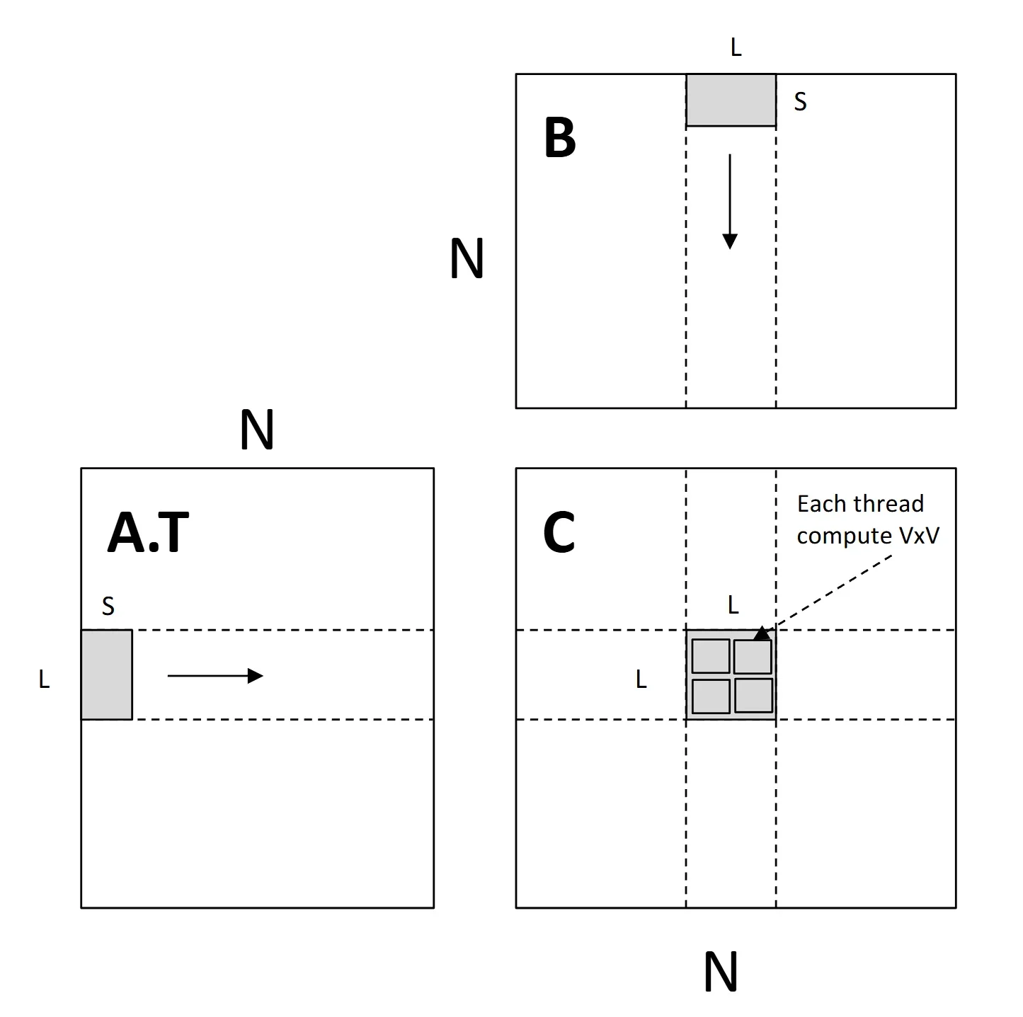
如上图所示,我们要计算的是两个长度为 N 的方阵之间的乘法,结果矩阵 C 会被分块为 (L,L) 的子矩阵,每个 block 负责计算一个子矩阵。
为了计算这个子矩阵,索引为 block_x, block_y 的 block 需要用到的数据为 A'=A[L*block_x:L*block_x+L,:] 和 B'=B[:,L*block_x:L*block_x+L]。A’ 和 B’ 可能比较大,因此在另一维度上按照长度 S 再次分为 N/S 块,分块后的 shape 分别为 (L,S) 和 (S,L),二者的矩阵乘法结果的 shape 为 (L,L),将 N/S 块累加即可得到该 block 负责的子矩阵的结果。
后文将使用矩阵的 shape 来指代该矩阵。
在计算单个 (L,S) 和 (S,L) 的乘法时,每个 block 都会将其对应的数据,即图中 A 和 B 的阴影部分,加载进 block 内线程共享的共享内存中。
通过外积计算单个 (L,S) 和 (S,L) 的乘法,该算法简单说就是从 (L,S) 任取一列,从 (S,L) 中任取一行,进行外积运算。将各种组合方式的外积结果累加,即可实现矩阵乘法。
单个外积运算由 block 内的线程共同完成,如图中所示,每个 thread 负责计算的就是 (V,V) 的更小的矩阵。具体来说,从 (L,S) 任取一列的 shape 为 (L,1),从 (S,L) 任取一行的 shape 为 (1,L),对二者按照长度为 V 再次进行分块,即分块为 (V,1) 和 (1,V)shape 的两个矩阵,然后由一个线程负责计算二者的外积,得到 shape 为 (V,V) 的结果。
以上就是理论课伪代码中提到的算法,将其改写为 CUDA 代码时需要考虑各种情况,有如下注意点:
- 理论中提到的需要分块的场景,在实践中可能存在不能完美切分,由余数的情况,需要判断是否越界;
- 每个 block 要计算的结果子矩阵是根据该 block 在 grid 中的位置确定的,每个 thread 要计算的外积的部分是根据其在 block 中的位置确定的;
- 理论中的 S 和 L 在代码中均取值为宏定义常量
TILE 4,V 取值为宏定义常量 V 2。
代码中写了比较详细的注释,这部分比较复杂,难以单纯通过文字讲明白,如有问题欢迎留言一起讨论。
  1
  2
  3
  4
  5
  6
  7
  8
  9
 10
 11
 12
 13
 14
 15
 16
 17
 18
 19
 20
 21
 22
 23
 24
 25
 26
 27
 28
 29
 30
 31
 32
 33
 34
 35
 36
 37
 38
 39
 40
 41
 42
 43
 44
 45
 46
 47
 48
 49
 50
 51
 52
 53
 54
 55
 56
 57
 58
 59
 60
 61
 62
 63
 64
 65
 66
 67
 68
 69
 70
 71
 72
 73
 74
 75
 76
 77
 78
 79
 80
 81
 82
 83
 84
 85
 86
 87
 88
 89
 90
 91
 92
 93
 94
 95
 96
 97
 98
 99
100
101
102
103
104
105
106
107
108
109
110
111
112
113
114
115
116
117
118
119
120
121
122
123
124
125
126
127
128
129
130
131
132
133
134
135
136
137
138
139
140
|
__global__ void MatmulKernel(const scalar_t* a, const scalar_t* b, scalar_t* c, uint32_t M, uint32_t N,
            uint32_t P){
#define V 2
#define TILE 4
  /**
   * 使用分块计算矩阵乘法,按照TILE大小分块
   * a: M x N
   * b: N x P
   */
  int block_x = blockIdx.x;
  int block_y = blockIdx.y;
  int thread_x = threadIdx.x;
  int thread_y = threadIdx.y;
  int thread_id = thread_x + thread_y * blockDim.x;
  int nthreads = blockDim.x * blockDim.y;
  // 每个block负责计算一个子矩阵的结果,具体来说,就是c[block_x*TILE: (block_x+1)*TILE, block_y*TILE: (block_y+1)*TILE]
  // 通过累加"outer product"的结果计算这个子矩阵,product的两个元素都是分块后行列子矩阵的一个stripe
  // 例如,a按行分块后每一块shape是(TILE, N),再取一个stripe的shape就是(TILE, TILE)
  // outer product每次的步长不是1,而是TILE

  __shared__ scalar_t a_shared[TILE][TILE];
  __shared__ scalar_t b_shared[TILE][TILE];
  scalar_t c_reg[V][V] = {0};
  scalar_t a_reg[V]={0}, b_reg[V]={0};


  for(int start=0; start<N; start+=TILE){
    __syncthreads();
    // 一共有TILE * TILE个元素要导入,每个线程平均负责(TILE * TILE+nthreads-1)/nthreads个元素
    // for (int i=0; i<(TILE * TILE+nthreads-1)/nthreads; i++){
    //   int idx = thread_id + i * nthreads; // 在shared中的索引
    //   int x = idx / TILE; // 在shared中的索引
    //   int y = idx % TILE; // 在shared中的索引
    //   // a_shared中的(x, y)相当于a中的(x+block_x*TILE, y+start)
    //   // b_shared中的(x, y)相当于b中的(x+start, y+block_y*TILE)
    //   if(x+block_x*TILE < M && y+start < N){
    //     a_shared[x][y] = a[(x+block_x*TILE)*N + y+start];
    //   }
    //   if(x+start < N && y+block_y*TILE < P){
    //     b_shared[x][y] = b[(x+start)*P + y+block_y*TILE];
    //   }
    // }
    for (int idx = thread_id; idx < TILE * TILE; idx += nthreads){
      int x = idx / TILE; // 在shared中的索引
      int y = idx % TILE; // 在shared中的索引
      // a_shared中的(x, y)相当于a中的(x+block_x*TILE, y+start)
      // b_shared中的(x, y)相当于b中的(x+start, y+block_y*TILE)
      if(x+block_x*TILE < M && y+start < N){
        a_shared[x][y] = a[(x+block_x*TILE)*N + y+start];
      }
      if(x+start < N && y+block_y*TILE < P){
        b_shared[x][y] = b[(x+start)*P + y+block_y*TILE];
      }
    }
    __syncthreads();
    // 接下来开始计算外积
    // 通过遍历a_shared的列和b_shared的行,也就是a_shared的第stripe_i行和b_shared的第stripe_i列
    int stripe_cnt = min(TILE, N-start);
    for(int stripe_i=0; stripe_i<stripe_cnt; stripe_i++){
    // 这个外积由nthreads负责计算,这个外积将stripe_a 和 stripe_b 按照连续的V行/列分块,由每个线程计算
    // 接下来把计算V*V的外积结果的要用的数据加载到寄存器数组中
      if(thread_x * V >= TILE || thread_y * V >= TILE)
        continue;
      for(int reg_x=0; reg_x<V; reg_x++){
        int shared_x = reg_x + thread_x * V;
        if(shared_x >= TILE){
          break;
        }
        a_reg[reg_x] = a_shared[shared_x][stripe_i];
        // b_reg[reg_x] = b_shared[stripe_i][shared_x];
      }
      for(int reg_y=0; reg_y<V; reg_y++){
        int shared_y = reg_y + thread_y * V;
        if(shared_y >= TILE){
          printf("quit: thread id: %d, shared_y: %d, TILE: %d\n", thread_id, shared_y, TILE);
          break;
        }
        // a_reg[reg_y] = a_shared[stripe_i][shared_y];
        b_reg[reg_y] = b_shared[stripe_i][shared_y];
      }
      for(int i=0; i<V; i++){
        for(int j=0; j<V; j++){
          // 这里“越界”可以不管吧?把c_reg放到结果中的时候再处理
          c_reg[i][j] += a_reg[i] * b_reg[j];
        }
      }
    }
  }

  // 把c_reg的结果写入到c中
  if(thread_x * V >= TILE || thread_y * V >= TILE)
    return;
  for(int i=0; i<V; i++){
    for(int j=0; j<V; j++){
      int x = block_x * TILE + thread_x * V + i;
      int y = block_y * TILE + thread_y * V + j;
      if(x < M && y < P){
        c[x*P + y] = c_reg[i][j];
      } else {
        break;
      }

    }
  }


}

void Matmul(const CudaArray& a, const CudaArray& b, CudaArray* out, uint32_t M, uint32_t N,
            uint32_t P) {
  /**
   * Multiply two (compact) matrices into an output (also comapct) matrix.  You will want to look
   * at the lecture and notes on GPU-based linear algebra to see how to do this.  Since ultimately
   * mugrade is just evaluating correctness, you _can_ implement a version that simply parallelizes
   * over (i,j) entries in the output array.  However, to really get the full benefit of this
   * problem, we would encourage you to use cooperative fetching, shared memory register tiling,
   * and other ideas covered in the class notes.  Note that unlike the tiled matmul function in
   * the CPU backend, here you should implement a single function that works across all size
   * matrices, whether or not they are a multiple of a tile size.  As with previous CUDA
   * implementations, this function here will largely just set up the kernel call, and you should
   * implement the logic in a separate MatmulKernel() call.
   *
   *
   * Args:
   *   a: compact 2D array of size m x n
   *   b: comapct 2D array of size n x p
   *   out: compact 2D array of size m x p to write the output to
   *   M: rows of a / out
   *   N: columns of a / rows of b
   *   P: columns of b / out
   */

  /// BEGIN SOLUTION
  // 结果的shape是M*P,每个block负责计算一个TILE*TILE的子矩阵
  dim3 grid_dim = dim3((M + TILE - 1) / TILE, (P + TILE - 1) / TILE, 1);
  dim3 block_dim = dim3(16, 16, 1);
  // dim3 block_dim = dim3(2, 2, 1);
  MatmulKernel<<<grid_dim, block_dim>>>(a.ptr, b.ptr, out->ptr, M, N, P);
  /// END SOLUTION
}
|
hw3 小结#
本 hw 主要内容是各算子 CPU 和 GPU 版本的底层实现,由于是第一次接触 CUDA 代码,在实现 GPU 版本的矩阵乘法的时候花了不少时间 Debug,调试到最后甚至要头疼昏睡过去。好在皇天不负苦心人,灵感一瞬间它就来了,谁懂这柳暗花明又一村的感觉。特别感谢 好友 为我讲解矩阵乘法的实现、大半夜不厌其烦地与我一起调试代码。
hw4#
本实验中,首先将实现一些算子,然后分别实现 CNN 和 RNN 网络,并在数据集上进行训练。
Part 1: ND Backend#
首先将 src/*、autograd.py、ndarray.py 文件中未实现的方法从之前的 hw 中复制过来,然后在 ops_*.py 中实现之前实现过的 op,大部分只要复制粘贴。
提一下我踩过的坑 :
autograd.py 中头文件为如下内容,以保证我们这里使用的后端是根据环境变量 NEEDLE_BACKEND 自动切换的,并且不为 NumPy 后端。
 1
 2
 3
 4
 5
 6
 7
 8
 9
10
11
12
13
14
|
import needle
# from .backend_numpy import Device, cpu, all_devices
from typing import List, Optional, NamedTuple, Tuple, Union
from collections import namedtuple
import numpy

from needle import init

# needle version
LAZY_MODE = False
TENSOR_COUNTER = 0

from .backend_selection import array_api, NDArray, default_device
from .backend_selection import Device, cpu, all_devices
|
- 在
ndarray.py 中 sum 和 max 规约函数是不支持指定多个轴的,需要修改之以便支持多个轴。
 1
 2
 3
 4
 5
 6
 7
 8
 9
10
11
12
13
14
15
16
17
18
19
20
21
22
23
24
25
26
27
|
def sum(self, axis=None, keepdims=False):
	if isinstance(axis, int):
		view, out = self.reduce_view_out(axis, keepdims=keepdims)
		self.device.reduce_sum(view.compact()._handle, out._handle, view.shape[-1])
	elif isinstance(axis, (tuple, list)):
		for axis_ in axis:
			view, out = self.reduce_view_out(axis_, keepdims=keepdims)
			self.device.reduce_sum(view.compact()._handle, out._handle, view.shape[-1])
	else:
		view, out = self.reduce_view_out(axis, keepdims=keepdims)
		self.device.reduce_sum(view.compact()._handle, out._handle, view.shape[-1])

	return out

def max(self, axis=None, keepdims=False):
	if isinstance(axis, int):
		view, out = self.reduce_view_out(axis, keepdims=keepdims)
		self.device.reduce_max(view.compact()._handle, out._handle, view.shape[-1])
	elif isinstance(axis, (tuple, list)):
		for axis_ in axis:
			view, out = self.reduce_view_out(axis_, keepdims=keepdims)
			self.device.reduce_max(view.compact()._handle, out._handle, view.shape[-1])
	else:
		view, out = self.reduce_view_out(axis, keepdims=keepdims)
		self.device.reduce_max(view.compact()._handle, out._handle, view.shape[-1])

	return out
|
- 在 reshape 之前,要调用 compact
- 在创建 Tensor 时,要确保其与其它数据的 device 相同
- 在
autograd.py 中,有一行代码为 __rsub__ = __sub__,其将 Tensor 的 rsub 方法重定向到了 sub 上,然而减法不具备交换律,该行代码是错误的。需要注释该行,并自行定义 rsub 函数。
1
2
|
def __rsub__(self, other):
	return needle.ops.AddScalar(other)(needle.ops.Negate()(self))
|
然后我们来实现新增的三个 op。
- tanh
tanh 在我们实现的 backend 中已经有对应的接口了,正向传播直接调用即可。tanh 反向传播公式为:
$$
\tanh^\prime(x) = 1-\tanh^2(x)
$$
反向传播中直接用 1 减去 node 的平方即可。需要注意,这里有一个上面提到的坑,也就是要自定义 rsub 函数。
 1
 2
 3
 4
 5
 6
 7
 8
 9
10
|
class Tanh(TensorOp):
    def compute(self, a):
        ### BEGIN YOUR SOLUTION
        return array_api.tanh(a)
        ### END YOUR SOLUTION

    def gradient(self, out_grad, node):
        ### BEGIN YOUR SOLUTION
        return out_grad * (1 - node ** 2)
        ### END YOUR SOLUTION
|
- stack
stack 函数是将多个相同 shape 的 Tensor 堆叠起来,并且会产生一个新的维度。正向传播实现的思路是先分配一个目标 shape 的 Tensor,然后通过赋值运算将他们放到目标位置。这里预分配时 Tensor 需要指定 device 与输入的 Tensor device 一致。反向传播调用逆运算 split。
 1
 2
 3
 4
 5
 6
 7
 8
 9
10
11
12
13
14
15
16
17
18
19
20
21
22
23
24
25
26
27
28
29
30
31
|
class Stack(TensorOp):
    def __init__(self, axis: int):
        """
        Concatenates a sequence of arrays along a new dimension.
        Parameters:
        axis - dimension to concatenate along
        All arrays need to be of the same size.
        """
        self.axis = axis

    def compute(self, args: TensorTuple) -> Tensor:
        ### BEGIN YOUR SOLUTION
        if len(args) > 0:
            shape = args[0].shape
            for arg in args:
                assert arg.shape == shape, "The shape of all tensors should be the same"
            ret_shape = list(shape)
            ret_shape.insert(self.axis, len(args))
            ret = array_api.empty(ret_shape, device=args[0].device)
            for i, arg in enumerate(args):
                slices = [slice(None)] * len(ret_shape)
                slices[self.axis] = i
                ret[tuple(slices)] = arg
            return ret
        ### END YOUR SOLUTION


    def gradient(self, out_grad, node):
        ### BEGIN YOUR SOLUTION
        return split(out_grad, self.axis)
        ### END YOUR SOLUTION
|
- split
split 方法是将指定的一个维度全部拆开,需要注意的是拆开之后的维度不需要 keep dim,也就是要进行一次 reshape 操作,而在 reshape 前是需要显式调用 compact 的。反向传播直接调用 stack 方法即可。
 1
 2
 3
 4
 5
 6
 7
 8
 9
10
11
12
13
14
15
16
17
18
19
20
21
22
23
24
25
26
27
28
29
30
|
class Split(TensorTupleOp):
    def __init__(self, axis: int):
        """
        Splits a tensor along an axis into a tuple of tensors.
        (The "inverse" of Stack)
        Parameters:
        axis - dimension to split
        """
        self.axis = axis

    def compute(self, A):
        ### BEGIN YOUR SOLUTION
        ret = []
        ret_shape = list(A.shape)
        ret_shape.pop(self.axis)
        for i in range(A.shape[self.axis]):
            slices = [slice(None)] * len(A.shape)
            slices[self.axis] = i
            ret.append((A[tuple(slices)]).compact().reshape(ret_shape))
        return tuple(ret)
        ### END YOUR SOLUTION

    def gradient(self, out_grad, node):
        ### BEGIN YOUR SOLUTION
        return stack(out_grad, self.axis)
        ### END YOUR SOLUTION


def split(a, axis):
    return Split(axis)(a)
|
Part 2: CIFAR-10 dataset#
在本 Part 中,将完成对 CIFAR-10 数据库的解析。首先从之前的 hw 中复制 python/needle/data/data_transforms.py 和 python/needle/data/data_basic.py 两个文件,并修改 data_basic 中 DataLoader::__next__ 方法为:
1
2
3
4
5
6
7
|
def __next__(self):
	if self.index >= len(self.ordering):
		raise StopIteration
	else:
		batch = [Tensor(x) for x in self.dataset[self.ordering[self.index]]]
		self.index += 1
		return batch
|
在之前 hw 中使用 Tensor.make_const 来实现,但其不会根据当前的 backend 自动切换 cached_data 的数据结构。
CIFAR-10 的数据格式参考 CIFAR-10 and CIFAR-100 datasets,简单来说,按照 batch, channel, height, width 的格式排列。__init__ 方法实现参考网站上已经给出的代码读取数据集,然后进行 reshape 和归一化的操作即可,另外两个方法可以直接写出来。
 1
 2
 3
 4
 5
 6
 7
 8
 9
10
11
12
13
14
15
16
17
18
19
20
21
22
23
24
25
26
27
28
29
30
31
32
33
34
35
36
37
38
39
40
41
42
43
44
45
46
47
|
class CIFAR10Dataset(Dataset):
    def __init__(
        self,
        base_folder: str,
        train: bool,
        p: Optional[int] = 0.5,
        transforms: Optional[List] = None
    ):
        """
        Parameters:
        base_folder - cifar-10-batches-py folder filepath
        train - bool, if True load training dataset, else load test dataset
        Divide pixel values by 255. so that images are in 0-1 range.
        Attributes:
        X - numpy array of images
        y - numpy array of labels
        """
        ### BEGIN YOUR SOLUTION
        train_names = ['data_batch_1', 'data_batch_2', 'data_batch_3', 'data_batch_4', 'data_batch_5']
        test_names = ['test_batch']
        names = train_names if train else test_names
        dicts = []
        for name in names:
            with open(os.path.join(base_folder, name), 'rb') as f:
                dicts.append(pickle.load(f, encoding='bytes'))
        self.X = np.concatenate([d[b'data'] for d in dicts], axis=0).reshape(-1, 3, 32, 32)
        self.X = self.X / 255.0
        self.y = np.concatenate([d[b'labels'] for d in dicts], axis=0)

        ### END YOUR SOLUTION

    def __getitem__(self, index) -> object:
        """
        Returns the image, label at given index
        Image should be of shape (3, 32, 32)
        """
        ### BEGIN YOUR SOLUTION
        return self.X[index], self.y[index]
        ### END YOUR SOLUTION

    def __len__(self) -> int:
        """
        Returns the total number of examples in the dataset
        """
        ### BEGIN YOUR SOLUTION
        return len(self.X)
        ### END YOUR SOLUTION
|
Part 3: Convolutional neural network#
在本 Part 中,我们将首先实现一些算子,然后实现一个 CNN 网络并在 CIFAR 数据集上进行训练。
- pad
pad 操作逻辑为:首先计算出 out 的 shape,创建一个大小为 shape 的全零 Tensor,然后通过切片将原矩阵赋值到对应位置:
1
2
3
4
5
6
|
def pad(self, axes):
	out_shape = tuple(self.shape[i] + axes[i][0] + axes[i][1] for i in range(len(self.shape)))
	out = self.device.full(out_shape, 0)
	slices = tuple(slice(axes[i][0], axes[i][0] + self.shape[i]) for i in range(len(self.shape)))
	out[slices] = self
	return out
|
- flip
很难解释为什么,但是 flip 操作通过负 strides 和正 offset 就可以实现。具体来说,将需要 flip 的维度的 stride 值取负,offset 值等于需要 flip 的维度的 strides 乘 shape-1 然后求和。可以结合代码理解上面这段话:
 1
 2
 3
 4
 5
 6
 7
 8
 9
10
11
12
13
14
15
16
17
18
19
20
21
22
23
24
25
26
27
28
|
# ndarray.py
def flip(self, axes):
	assert isinstance(axes, tuple), "axes must be a tuple"

	strides = tuple(self.strides[i] if i not in axes else -self.strides[i] for i in range(len(self.shape)))
	sum = __builtins__["sum"]
	offset = sum((self.shape[i] - 1) * self.strides[i] for i in range(len(self.shape)) if i in axes)
	out = NDArray.make(self.shape, strides=strides, device=self.device, handle=self._handle, offset=offset).compact()
	return out

# ops_mathematic.py
class Flip(TensorOp):
    def __init__(self, axes: Optional[tuple] = None):
        if isinstance(axes, int):
            axes = (axes,)
        if isinstance(axes, list):
            axes = tuple(axes)
        self.axes = axes

    def compute(self, a):
        ### BEGIN YOUR SOLUTION
        return array_api.flip(a, self.axes)
        ### END YOUR SOLUTION

    def gradient(self, out_grad, node):
        ### BEGIN YOUR SOLUTION
        return flip(out_grad, self.axes)
        ### END YOUR SOLUTION
|
通过操纵 offset 和 strides 实现 flip 在数学角度应该是可以证明的,此处不表。
- dilate/undilate
dilate 操作之前没有接触过,但下边的公式很形象:
$$
\begin{bmatrix}
1 & 2 \\
3 & 4
\end{bmatrix}
\Longrightarrow
\begin{bmatrix}
1 & 0 & 2 & 0 \\
0 & 0 & 0 & 0 \\
3 & 0 & 4 & 0 \\
0 & 0 & 0 & 0
\end{bmatrix}
$$
参数 dilation 就是 0 的个数。
这个函数的实现思路与 flip 非常接近,先计算 out 的 shape,然后创建空矩阵,然后通过切片选择目标元素:
 1
 2
 3
 4
 5
 6
 7
 8
 9
10
11
12
13
14
15
16
17
18
19
20
21
22
23
24
25
26
27
28
29
30
31
32
33
34
35
36
37
38
39
40
41
42
43
44
45
46
47
48
49
50
51
52
53
54
55
56
57
58
|
class Dilate(TensorOp):
    def __init__(self, axes: tuple, dilation: int):
        self.axes = axes
        self.dilation = dilation

    def compute(self, a):
        ### BEGIN YOUR SOLUTION
        if self.dilation == 0:
            return a
        out_shape = list(a.shape)
        for i in self.axes:
            out_shape[i] *= self.dilation + 1
        out = array_api.full(out_shape, 0, device=a.device)
        slices = [slice(None)] * len(a.shape)
        for dim in self.axes:
            slices[dim] = slice(None, None, self.dilation+1)
        out[tuple(slices)] = a
        return out
        ### END YOUR SOLUTION

    def gradient(self, out_grad, node):
        ### BEGIN YOUR SOLUTION
        return undilate(out_grad, self.axes, self.dilation)
        ### END YOUR SOLUTION


def dilate(a, axes, dilation):
    return Dilate(axes, dilation)(a)


class UnDilate(TensorOp):
    def __init__(self, axes: tuple, dilation: int):
        self.axes = axes
        self.dilation = dilation

    def compute(self, a):
        ### BEGIN YOUR SOLUTION
        if self.dilation == 0:
            return a
        out_shape = list(a.shape)
        for i in self.axes:
            out_shape[i] //= self.dilation + 1
        out = array_api.empty(out_shape, device=a.device)
        slices = [slice(None)] * len(a.shape)
        for dim in self.axes:
            slices[dim] = slice(None, None, self.dilation+1)
        out = a[tuple(slices)]
        return out
        ### END YOUR SOLUTION

    def gradient(self, out_grad, node):
        ### BEGIN YOUR SOLUTION
        return dilate(out_grad, self.axes, self.dilation)
        ### END YOUR SOLUTION


def undilate(a, axes, dilation):
    return UnDilate(axes, dilation)(a)
|
dilate 和 undilate 互为逆运算,在计算梯度时互相调用即可。
- conv
首先处理 padding,不难发现,padding 和 conv 之间具有结合性,即如下两行代码是等价的:
1
2
3
|
conv(X, W, padding=n)

conv(pad(X, n), W, padding=0)
|
因此,第一步就是将 X 进行 pad,作为新的 X。后面通过 im2col 技术和操作 strides 将 X 和 W 向量化,通过矩阵乘法来实现卷积。上述原理见课程笔记:《CMU 10-414 deep learning system》学习笔记 | 周鑫的个人博客。
反向传播推导见博文:2d 卷积梯度推导与实现 | 周鑫的个人博客
实现 Conv 的代码中使用了较多的 permute 重排操作,如果用 transpose 来实现重排太麻烦了,倒不如直接实现个重排的 TensorOp:
 1
 2
 3
 4
 5
 6
 7
 8
 9
10
11
12
13
14
15
16
17
18
19
20
|
class Permute(TensorOp):
    def __init__(self, axes: tuple):
        self.axes = axes

    def compute(self, a):
        ### BEGIN YOUR SOLUTION
        return a.compact().permute(self.axes)
        ### END YOUR SOLUTION

    def gradient(self, out_grad, node):
        ### BEGIN YOUR SOLUTION
        a = node.inputs[0]
        index = [0] * len(self.axes)
        for i in range(len(self.axes)):
            index[self.axes[i]] = i
        return permute(out_grad, tuple(index))
        ### END YOUR SOLUTION

def permute(a, axes):
    return Permute(axes)(a)
|
最终实现的代码为:
 1
 2
 3
 4
 5
 6
 7
 8
 9
10
11
12
13
14
15
16
17
18
19
20
21
22
23
24
25
26
27
28
29
30
31
32
33
34
35
36
37
38
39
40
41
42
43
44
45
46
47
48
49
50
51
52
53
|
class Conv(TensorOp):
    def __init__(self, stride: Optional[int] = 1, padding: Optional[int] = 0):
        self.stride = stride
        self.padding = padding

    def compute(self, A, B):
        ### BEGIN YOUR SOLUTION
        assert len(A.shape) == 4, "The input tensor should be 4D"
        assert len(B.shape) == 4, "The kernel tensor should be 4D"
        A = A.compact()
        B = B.compact()
        batch_size, in_height, in_width, in_channel = A.shape
        bs, hs, ws, cs = A.strides
        kernel_height, kernel_width, in_channel, out_channel = B.shape


        pad_A = A.pad(((0, 0), (self.padding, self.padding), (self.padding, self.padding), (0, 0))).compact()
        batch_size, in_height, in_width, in_channel = pad_A.shape
        bs, hs, ws, cs = pad_A.strides
        receiptive_field_shape = (batch_size, (in_height - kernel_height) // self.stride + 1, (in_width - kernel_width) // self.stride + 1, kernel_height, kernel_width, in_channel)
        receiptive_field_strides = (bs, hs * self.stride, ws * self.stride, hs, ws, cs)
        receiptive_field = pad_A.as_strided(receiptive_field_shape, receiptive_field_strides).compact()
        reveiptive_vector = receiptive_field.reshape((receiptive_field.size //(kernel_height * kernel_width * in_channel), kernel_height * kernel_width * in_channel)).compact()
        kernel_vector = B.reshape((kernel_height * kernel_width * in_channel, out_channel)).compact()
        out = reveiptive_vector @ kernel_vector
        out = out.reshape((batch_size, (in_height - kernel_height) // self.stride + 1, (in_width - kernel_width) // self.stride + 1, out_channel)).compact()
        return out
        ### END YOUR SOLUTION

    def gradient(self, out_grad, node):
        ### BEGIN YOUR SOLUTION
        X, W = node.inputs
        s, _, _, _ = W.shape

        # 计算X_grad
        W_flipped = flip(W, (0, 1))
        W_flipped_permuted = transpose(W_flipped, (2, 3)) # transpose 只支持两个维度的交换
        outgrad_dilated = dilate(out_grad, (1, 2), self.stride - 1)
        X_grad = conv(outgrad_dilated, W_flipped_permuted, padding=s - 1 - self.padding)

        # 计算W_grad
        # outgrad_dilated = dilate(out_grad, (1, 2), self.stride - 1)
        outgrad_dilated_permuted = permute(outgrad_dilated, (1, 2, 0, 3))
        X_permuted = permute(X, (3, 1, 2, 0))
        W_grad = conv(X_permuted, outgrad_dilated_permuted, padding=self.padding)
        W_grad = permute(W_grad, (1, 2, 0, 3))
        return X_grad, W_grad
        ### END YOUR SOLUTION


def conv(a, b, stride=1, padding=1):
    return Conv(stride, padding)(a, b)
|
- nn.Conv
这里将实现一个卷积层。由如下要求:输入输出的格式为 (N,C,H,W),padding 应满足当 stride=1 时,输出不缩水,支持 bias 项。
首先修改 Kaming uniform 的实现,使之支持对卷积核的初始化。增加一个逻辑,根据参数 shape 是否为 None,在调用 rand 函数时传入不同的形状即可:
 1
 2
 3
 4
 5
 6
 7
 8
 9
10
11
12
|
def kaiming_uniform(fan_in, fan_out, shape=None, nonlinearity="relu", **kwargs):
    assert nonlinearity == "relu", "Only relu supported currently"
    ### BEGIN YOUR SOLUTION
    if nonlinearity == "relu":
        gain = math.sqrt(2)
    ### BEGIN YOUR SOLUTION
    bound = gain * math.sqrt(3 / fan_in)
    if shape is None:
        return rand(fan_in, fan_out, low=-bound, high=bound, **kwargs)
    else:
        return rand(*shape, low=-bound, high=bound, **kwargs)
    ### END YOUR SOLUTION
|
hw4 的代码中,对于 NDArray.sum 的实现有问题,当求和的维度指定为空 tuple 时,其不应该进行求和操作,但原始代码无法正确处理这种情况,需要参数 axis 类型为 list 或者 tuple 的分支进行额外的判断,如果为空 list 或者 tuple,输出等于输入:
 1
 2
 3
 4
 5
 6
 7
 8
 9
10
11
12
13
14
15
|
def sum(self, axis=None, keepdims=False):
	if isinstance(axis, int):
		view, out = self.reduce_view_out(axis, keepdims=keepdims)
		self.device.reduce_sum(view.compact()._handle, out._handle, view.shape[-1])
	elif isinstance(axis, (tuple, list)):
		if len(axis) == 0:
			out = self
		for axis_ in axis:
			view, out = self.reduce_view_out(axis_, keepdims=keepdims)
			self.device.reduce_sum(view.compact()._handle, out._handle, view.shape[-1])
	else:
		view, out = self.reduce_view_out(axis, keepdims=keepdims)
		self.device.reduce_sum(view.compact()._handle, out._handle, view.shape[-1])

	return out
|
万事俱备,卷积层的实现调用上边的函数即可。初始化的部分,根据文档描述初始化好权重和偏执项。对于步长为 1 的卷积,卷积结果会缩水 k-1 行 k-1 列,为了确保 shape 不变,卷积时四周要 pad (k-1)/2,又由于传统上 k 为奇数,因此等价于 pad k/2。
前向传播的部分,首先将 X 重排为 NHWC 的格式,然后加上卷积层。如果由偏执项,则将其广播后再加到结果中,最后将结果重排为 NCHW 格式返回即可。完整代码为:
 1
 2
 3
 4
 5
 6
 7
 8
 9
10
11
12
13
14
15
16
17
18
19
20
21
22
23
24
25
26
27
28
29
30
31
32
33
34
35
36
|
class Conv(Module):
    """
    Multi-channel 2D convolutional layer
    IMPORTANT: Accepts inputs in NCHW format, outputs also in NCHW format
    Only supports padding=same
    No grouped convolution or dilation
    Only supports square kernels
    """
    def __init__(self, in_channels, out_channels, kernel_size, stride=1, bias=True, device=None, dtype="float32"):
        super().__init__()
        if isinstance(kernel_size, tuple):
            kernel_size = kernel_size[0]
        if isinstance(stride, tuple):
            stride = stride[0]
        self.in_channels = in_channels
        self.out_channels = out_channels
        self.kernel_size = kernel_size
        self.stride = stride

        ### BEGIN YOUR SOLUTION
        self.weight = Parameter(init.kaiming_uniform(self.in_channels, self.out_channels, shape=(kernel_size, kernel_size, in_channels, out_channels), device=device, dtype=dtype))
        bias_bound = 1.0 / np.sqrt(in_channels * kernel_size * kernel_size)
        self.bias = Parameter(init.rand(out_channels, low=-bias_bound, high=bias_bound, device=device, dtype=dtype)) if bias else None
        self.padding = kernel_size // 2
        ### END YOUR SOLUTION

    def forward(self, x: Tensor) -> Tensor:
        ### BEGIN YOUR SOLUTION
        # convert NCHW to NHWC
        x = ops.permute(x, [0, 2, 3, 1])
        conv_x = ops.conv(x, self.weight, stride=self.stride, padding=self.padding)
        if self.bias is not None:
            broadcasted_bias = ops.broadcast_to(ops.reshape(self.bias, (1, 1, 1, self.out_channels)), conv_x.shape)
            conv_x = conv_x + broadcasted_bias
        out = ops.permute(conv_x, [0, 3, 1, 2])
        return out
|
- ResNet 9
在实现 TensorOp 的子类时,如果需要初始化 Tensor,一定要指定 device。之前在实现 ReLU 生成 mask 时没有指定 device,将导致反向传播失败,这里对其进行修改:
 1
 2
 3
 4
 5
 6
 7
 8
 9
10
11
|
class ReLU(TensorOp):
    def compute(self, a):
        ### BEGIN YOUR SOLUTION
        return array_api.maximum(a, 0)
        ### END YOUR SOLUTION

    def gradient(self, out_grad, node):
        ### BEGIN YOUR SOLUTION
        relu_mask = Tensor(node.inputs[0].cached_data > 0, device=node.inputs[0].device)
        return out_grad * relu_mask
        ### END YOUR SOLUTION
|
同样,之前在实现 SoftmaxLoss 生成 one hot 时也没有指定 device,这里需要修改:
1
2
3
4
5
6
7
8
|
class SoftmaxLoss(Module):
    def forward(self, logits: Tensor, y: Tensor):
        ### BEGIN YOUR SOLUTION
        batch_size, label_size = logits.shape
        one_hot_y = init.one_hot(label_size, y, device=logits.device)
        true_logits = ops.summation(logits * one_hot_y, axes=(1,))
        return (ops.logsumexp(logits, axes=(1, )) - true_logits).sum()/batch_size
        ### END YOUR SOLUTION
|
此外,还发现在 reshape 操作可能没有调用 compact,这里直接修改其实现,在调用 array_api 前进行 compact 操作:
 1
 2
 3
 4
 5
 6
 7
 8
 9
10
11
12
13
14
15
|
class Reshape(TensorOp):
    def __init__(self, shape):
        self.shape = shape

    def compute(self, a):
        ### BEGIN YOUR SOLUTION
        expect_size = 1
        for i in self.shape:
            expect_size *= i
        real_size = 1
        for i in a.shape:
            real_size *= i
        assert expect_size == real_size , "The reshape size is not compatible"
        return array_api.reshape(a.compact(), self.shape)
        ### END YOUR SOLUTION
|
经过一番小修小补,我们的代码已经相当健壮,足以完成这个 ResNet 9🎉。ResNet 9 网络架构如下所示。写代码的过程中有些漏洞咱也没必要妄自菲薄,毕竟这么厉害的两位大佬也难免有笔误的地方。下图中的 ResNet 9 有一层网络架构写错了,已在原图中指出。
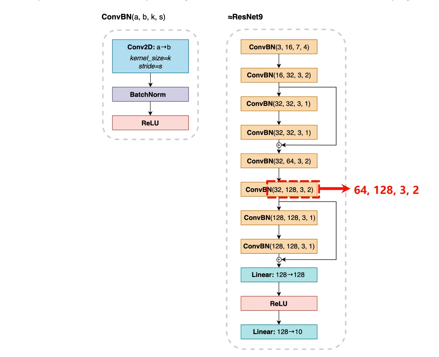
首先来实现 ConvBN,传入的四个参数以此为 channels_in,channels_out,kernel_size 和 stride。hw4 的框架代码中提供了 BatchNorm2d,在拷贝 nn_basic.py 文件时不要直接覆盖。剩余的实现很简单,根据示意图搭积木,运行后哪里报 Not Implemented Error 就补哪里,完整代码为:
 1
 2
 3
 4
 5
 6
 7
 8
 9
10
11
12
13
14
15
16
17
18
19
20
21
22
23
24
25
26
27
28
29
30
31
32
33
34
35
36
37
38
39
40
41
|
class ResNet9(ndl.nn.Module):
    def __init__(self, device=None, dtype="float32"):
        super().__init__()
        bias = True
        ### BEGIN YOUR SOLUTION ###
        self.conv1 = ConvBN(3, 16, 7, 4, bias=bias, device=device, dtype=dtype)
        self.conv2 = ConvBN(16, 32, 3, 2, bias=bias, device=device, dtype=dtype)
        self.res = ndl.nn.Residual(
            ndl.nn.Sequential(
                ConvBN(32, 32, 3, 1, bias=bias, device=device, dtype=dtype),
                ConvBN(32, 32, 3, 1, bias=bias, device=device, dtype=dtype)
            )
        )
        self.conv3 = ConvBN(32, 64, 3, 2, bias=bias, device=device, dtype=dtype)
        self.conv4 = ConvBN(64, 128, 3, 2, bias=bias, device=device, dtype=dtype)
        self.res2 = ndl.nn.Residual(
            ndl.nn.Sequential(
                ConvBN(128, 128, 3, 1, bias=bias, device=device, dtype=dtype),
                ConvBN(128, 128, 3, 1, bias=bias, device=device, dtype=dtype)
            )
        )
        self.flatten = ndl.nn.Flatten()
        self.linear = ndl.nn.Linear(128, 128, bias=bias, device=device, dtype=dtype)
        self.relu = ndl.nn.ReLU()
        self.linear2 = ndl.nn.Linear(128, 10, bias=bias, device=device, dtype=dtype)
        ### END YOUR SOLUTION

    def forward(self, x):
        ### BEGIN YOUR SOLUTION
        x = self.conv1(x)
        x = self.conv2(x)
        x = self.res(x)
        x = self.conv3(x)
        x = self.conv4(x)
        x = self.res2(x)
        x = self.flatten(x)
        x = self.linear(x)
        x = self.relu(x)
        x = self.linear2(x)
        return x
        ### END YOUR SOLUTION
|
很遗憾,上述代码在我的设备上并不能通过 ResNet 9 的测试点,误差为 0.09,远超 tolerance 0.01。但其又能通过后续在 CIFAR 10 训练集上训练 2 epoches 的测试点,且误差为 5e-5,远小于 tolerance 0.01。怀疑前一个测试点数据有问题。
Part 4: Recurrent neural network#
- RNN Cell
RNN cell 似乎没有什么坑,照着文档初始化参数,照着公式进行正向传播:
 1
 2
 3
 4
 5
 6
 7
 8
 9
10
11
12
13
14
15
16
17
18
19
20
21
22
23
24
|
class RNNCell(Module):
    def __init__(self, input_size, hidden_size, bias=True, nonlinearity='tanh', device=None, dtype="float32"):
        super().__init__()
        ### BEGIN YOUR SOLUTION
        bound = 1 / np.sqrt(hidden_size)
        self.W_ih = Parameter(init.rand(input_size, hidden_size, low=-bound, high=bound, device=device, dtype=dtype))
        self.W_hh = Parameter(init.rand(hidden_size, hidden_size, low=-bound, high=bound, device=device, dtype=dtype))
        self.bias_ih = Parameter(init.rand(hidden_size, low=-bound, high=bound, device=device, dtype=dtype)) if bias else None
        self.bias_hh = Parameter(init.rand(hidden_size, low=-bound, high=bound, device=device, dtype=dtype)) if bias else None
        self.nonlinearity = ops.tanh if nonlinearity == 'tanh' else ops.relu
        ### END YOUR SOLUTION

    def forward(self, X, h=None):
        ### BEGIN YOUR SOLUTION
        if h is None:
            h = init.zeros(X.shape[0], self.W_hh.shape[0], device=X.device, dtype=X.dtype)
        Z = X@self.W_ih + h@self.W_hh
        if self.bias_ih:
            bias = self.bias_ih + self.bias_hh
            bias = bias.reshape((1, bias.shape[0]))
            bias = bias.broadcast_to(Z.shape)
            Z += bias
        return self.nonlinearity(Z)
        ### END YOUR SOLUTION
|
- RNN
本节任务是完成一个多层 RNN,即堆叠在一起的 RNN,如下图所示。参数中 num_layers 指定了层数,input_size 指的是最下面那层 RNN 的输入的 x 的 size,除底层之外的 cell 的输入都是前一层的输入,即它们的 input_size = hidden_size
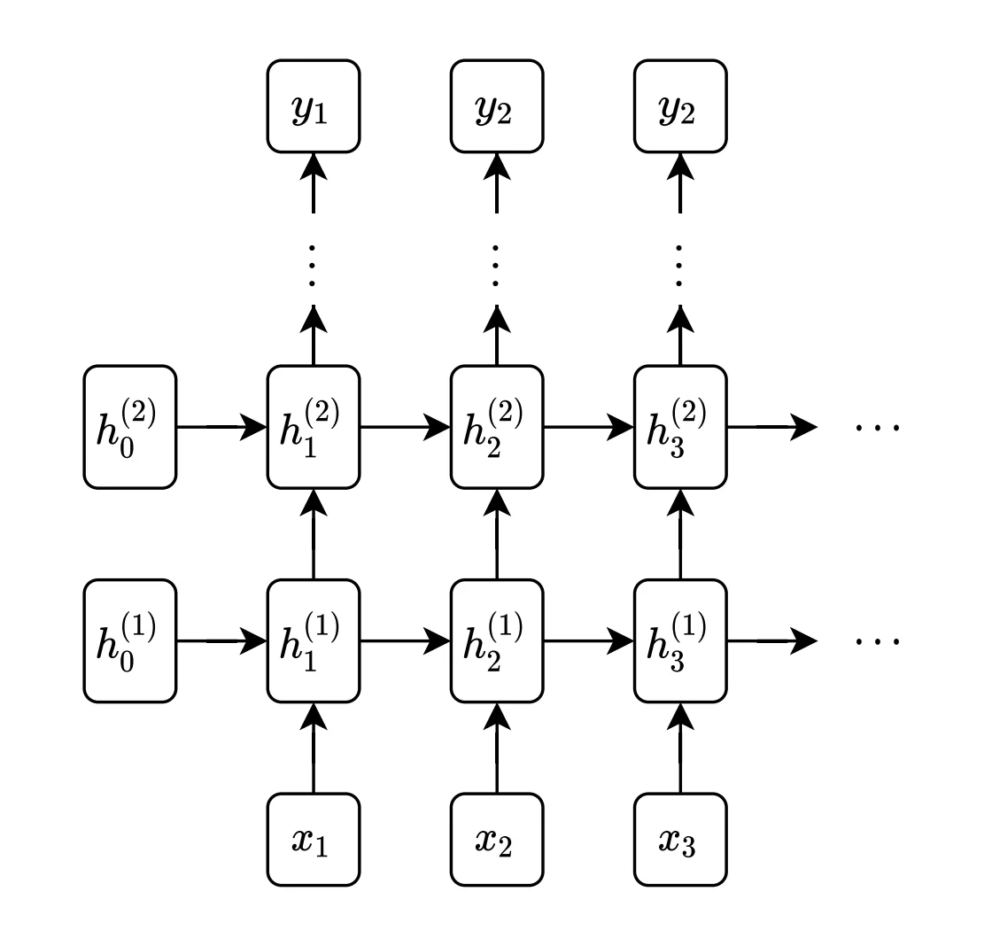
由上图,可知每一层的输入都是在变化的,因此考虑维护一个 X_input 列表用于存储当前没计算的 cell 的垂直输入。同样,维护一个 h_input 列表存储当前没计算的 cell 的水平输入。具体来说,当计算的 cell 编号为 $h_i^j$ 时,其用到的输入为 X_input[i] 和 h_input[j],同时计算结束后 X_input[j] 和 h_input[j] 都要更新为该节点的输出。
对于这个堆叠在一起的 RNN,可以采用从左往右、从下到上,或者从下到上、从左往右的计算方式。我采用的是先垂直再水平的计算顺序。
模型最后要返回两个变量,一个是最后一层的输出 output,即示意图中的 y 的集合,不难发现最后一层的输出就是最后一层的后一层(假设存在)的垂直输入,即我们一直在维护的 X_input。另一个要返回的变量是最后一列隐藏层,同样,这就是我们一直在维护的水平输入 h_input。水到渠成。
需要注意,Tensor 没有实现 getitem 和 setitem 方法,需要切片存取的时候调用之前实现的 split 和 stack 方法即可。
完整代码为:
 1
 2
 3
 4
 5
 6
 7
 8
 9
10
11
12
13
14
15
16
17
18
19
20
21
22
23
24
25
26
27
28
|
class RNN(Module):
    def __init__(self, input_size, hidden_size, num_layers=1, bias=True, nonlinearity='tanh', device=None, dtype="float32"):
        super().__init__()
        ### BEGIN YOUR SOLUTION
        self.rnn_cells = []
        self.rnn_cells.append(RNNCell(input_size, hidden_size, bias, nonlinearity, device, dtype))
        for i in range(1, num_layers):
            self.rnn_cells.append(RNNCell(hidden_size, hidden_size, bias, nonlinearity, device, dtype))
        ### END YOUR SOLUTION

    def forward(self, X, h0=None):
        ### BEGIN YOUR SOLUTION
        seq_len = X.shape[0]
        layer_num = len(self.rnn_cells)
        if h0 is None:
            h0 = init.zeros(len(self.rnn_cells), X.shape[1], self.rnn_cells[0].W_hh.shape[0], device=X.device, dtype=X.dtype)
        h_input = list(ops.split(h0, 0)) # list length = num_layers, element shape = (bs, hidden_size)
        X_input = list(ops.split(X, 0)) # list length = seq_len, element shape = (bs, input_size)
        for i in range(seq_len):
            for j in range(layer_num):
                X_input[i] = self.rnn_cells[j](X_input[i], h_input[j])
                h_input[j] = X_input[i]
        output = ops.stack(X_input, 0) # output features of last layer == input X of last+1 layer
        h_n = ops.stack(h_input, 0)
        return output, h_n


        ### END YOUR SOLUTION
|
Part 5: LSTM#
本章节将实现 LSTM,LSTM 和上边的 RNN 逻辑相同,照抄公式,这里直接放出代码:
 1
 2
 3
 4
 5
 6
 7
 8
 9
10
11
12
13
14
15
16
17
18
19
20
21
22
23
24
25
26
27
28
29
30
31
32
33
34
35
36
37
38
39
40
41
42
43
44
45
46
47
48
49
50
51
52
53
54
55
56
57
58
59
60
61
62
63
64
65
66
67
68
69
70
71
72
73
|
class LSTMCell(Module):
    def __init__(self, input_size, hidden_size, bias=True, device=None, dtype="float32"):
        super().__init__()
        ### BEGIN YOUR SOLUTION
        bound = 1.0 / np.sqrt(hidden_size)
        self.W_ih = Parameter(init.rand(input_size, 4*hidden_size, low=-bound, high=bound, device=device, dtype=dtype))
        self.W_hh = Parameter(init.rand(hidden_size, 4*hidden_size, low=-bound, high=bound, device=device, dtype=dtype))
        self.bias_ih = Parameter(init.rand(4*hidden_size, low=-bound, high=bound, device=device, dtype=dtype)) if bias else None
        self.bias_hh = Parameter(init.rand(4*hidden_size, low=-bound, high=bound, device=device, dtype=dtype)) if bias else None
        self.sigmoid = Sigmoid()
        ### END YOUR SOLUTION


    def forward(self, X, h=None):
        ### BEGIN YOUR SOLUTION
        bs = X.shape[0]
        hidden_size = self.W_hh.shape[0]
        if h is None:
            h0 = init.zeros(bs, hidden_size, device=X.device, dtype=X.dtype)
            c0 = init.zeros(bs, hidden_size, device=X.device, dtype=X.dtype)
        else:
            h0, c0 = h
        Z = X@self.W_ih + h0@self.W_hh # [bs, 4*hidden_size]
        if self.bias_ih:
            bias = self.bias_ih + self.bias_hh
            bias = bias.reshape((1, bias.shape[0]))
            bias = bias.broadcast_to(Z.shape)
            Z += bias
        stripes = list(ops.split(Z, 1))
        i = self.sigmoid(ops.stack(stripes[0: hidden_size], 1))
        f = self.sigmoid(ops.stack(stripes[hidden_size: 2*hidden_size], 1))
        g = ops.tanh(ops.stack(stripes[2*hidden_size: 3*hidden_size], 1))
        o = self.sigmoid(ops.stack(stripes[3*hidden_size: 4*hidden_size], 1))
        c = f * c0 + i * g
        h = o * ops.tanh(c)
        return h, c

        ### END YOUR SOLUTION


class LSTM(Module):
    def __init__(self, input_size, hidden_size, num_layers=1, bias=True, device=None, dtype="float32"):
        super().__init__()
        ### BEGIN YOUR SOLUTION
        self.lstm_cells = []
        self.lstm_cells.append(LSTMCell(input_size, hidden_size, bias, device, dtype))
        for i in range(1, num_layers):
            self.lstm_cells.append(LSTMCell(hidden_size, hidden_size, bias, device, dtype))
        ### END YOUR SOLUTION

    def forward(self, X, h=None):
        ### BEGIN YOUR SOLUTION
        seq_len, bs, _ = X.shape
        num_layers = len(self.lstm_cells)
        hidden_size = self.lstm_cells[0].W_hh.shape[0]
        if h is None:
            h0 = init.zeros(num_layers, bs, hidden_size, device=X.device, dtype=X.dtype)
            c0 = init.zeros(num_layers, bs, hidden_size, device=X.device, dtype=X.dtype)
        else:
            h0, c0 = h
        h_input = list(ops.split(h0, 0))
        c_input = list(ops.split(c0, 0))
        X_input = list(ops.split(X, 0))
        for i in range(seq_len):
            for j in range(num_layers):
                X_input[i], c_input[j] = self.lstm_cells[j](X_input[i], (h_input[j], c_input[j]))
                h_input[j] = X_input[i]
        output = ops.stack(X_input, 0)
        h_n = ops.stack(h_input, 0)
        c_n = ops.stack(c_input, 0)
        return output, (h_n, c_n)

        ### END YOUR SOLUTION
|
Part 6: Penn Treebank dataset#
- Dictionary
这个类的作用是构建一个从 word 到 id 双向映射的字典,word2idx 通过读取 dict 来实现,idx2word 通过访问 list 来实现:
 1
 2
 3
 4
 5
 6
 7
 8
 9
10
11
12
13
14
15
16
17
|
class Dictionary(object):
    def __init__(self):
        self.word2idx = {}
        self.idx2word = []

    def add_word(self, word):
        ### BEGIN YOUR SOLUTION
        if self.word2idx.get(word) is None:
            self.word2idx[word] = len(self.idx2word)
            self.idx2word.append(word)
        return self.word2idx[word]
        ### END YOUR SOLUTION

    def __len__(self):
        ### BEGIN YOUR SOLUTION
        return len(self.idx2word)
        ### END YOUR SOLUTION
|
- Corpus
这个类的作用类似于 DataLoader,从文件读取原始数据,通过 Dictionary 将其 tokenize,提供 batchify 将其分割为 batch(这个 batch 指的是输入的 x 中同时存在好几个句子),提供 get_batch 方法将单个句子分割为 batch(这是由于 lstm 的水平深度有限,最多同时接受这么多输入)。
具体实现时参考 docstring 描述即可,由示意图,一目了然。完整代码为:
 1
 2
 3
 4
 5
 6
 7
 8
 9
10
11
12
13
14
15
16
17
18
19
20
21
22
23
24
25
26
27
28
29
30
31
32
33
34
35
36
37
|
class Corpus(object):
    def __init__(self, base_dir, max_lines=None):
        self.dictionary = Dictionary()
        self.train = self.tokenize(os.path.join(base_dir, 'train.txt'), max_lines)
        self.test = self.tokenize(os.path.join(base_dir, 'test.txt'), max_lines)

    def tokenize(self, path, max_lines=None):
        ### BEGIN YOUR SOLUTION
        with open(path, 'r') as f:
            ids = []
            line_idx = 0
            for line in f:
                if max_lines is not None and line_idx >= max_lines:
                    break
                words = line.split() + ['<eos>']
                for word in words:
                    ids.append(self.dictionary.add_word(word))
                line_idx += 1
        return ids
        ### END YOUR SOLUTION


def batchify(data, batch_size, device, dtype):
    ### BEGIN YOUR SOLUTION
    data_len = len(data)
    nbatch = data_len // batch_size
    data = data[:nbatch * batch_size]
    return np.array(data).reshape(batch_size, -1).T
    ### END YOUR SOLUTION


def get_batch(batches, i, bptt, device=None, dtype=None):
    ### BEGIN YOUR SOLUTION
    data = batches[i: i + bptt, :]
    target = batches[i + 1: i + 1 + bptt, :]
    return Tensor(data, device=device, dtype=dtype), Tensor(target.flatten(), device=device, dtype=dtype)
    ### END YOUR SOLUTION
|
Part 7: Training a word-level language model#
这里有个大坑,ndarray 实现的矩阵乘法不支持批量矩乘,如果由三维矩阵乘二维的情况,需要手动 reshape 再乘,再 reshape 回去。
- Embedding
这个 Module 的作用是将 token 进行一次线性变换,这个操作涉及到批量矩乘:
 1
 2
 3
 4
 5
 6
 7
 8
 9
10
11
12
13
14
15
|
class Embedding(Module):
    def __init__(self, num_embeddings, embedding_dim, device=None, dtype="float32"):
        super().__init__()
        ### BEGIN YOUR SOLUTION
        self.weight = Parameter(init.randn(num_embeddings, embedding_dim, device=device, dtype=dtype))
        ### END YOUR SOLUTION

    def forward(self, x: Tensor) -> Tensor:
        ### BEGIN YOUR SOLUTION
        one_hot = init.one_hot(self.weight.shape[0], x, device=x.device, dtype=x.dtype)
        seq_len, bs, num_embeddings = one_hot.shape
        one_hot = one_hot.reshape((seq_len*bs, num_embeddings))

        return ops.matmul(one_hot, self.weight).reshape((seq_len, bs, self.weight.shape[1]))
        ### END YOUR SOLUTION
|
- LanguageModel
搭积木,同样设计批量矩乘:
 1
 2
 3
 4
 5
 6
 7
 8
 9
10
11
12
13
14
15
16
17
18
19
20
21
22
|
class LanguageModel(nn.Module):
    def __init__(self, embedding_size, output_size, hidden_size, num_layers=1,
                 seq_model='rnn', device=None, dtype="float32"):
        super(LanguageModel, self).__init__()
        ### BEGIN YOUR SOLUTION
        self.embedding = nn.Embedding(output_size, embedding_size, device=device, dtype=dtype)
        if seq_model == 'rnn':
            self.model = nn.RNN(embedding_size, hidden_size, num_layers, device=device, dtype=dtype)
        elif seq_model == 'lstm':
            self.model = nn.LSTM(embedding_size, hidden_size, num_layers, device=device, dtype=dtype)
        self.linear = nn.Linear(hidden_size, output_size, device=device, dtype=dtype)
        ### END YOUR SOLUTION

    def forward(self, x, h=None):
        ### BEGIN YOUR SOLUTION
        x = self.embedding(x) # (seq_len, bs, embedding_size)
        out, h = self.model(x, h)
        seq_len, bs, hidden_size = out.shape
        out = out.reshape((seq_len * bs, hidden_size))
        out = self.linear(out)
        return out, h
        ### END YOUR SOLUTION
|
- epoch_general_ptb
流程和 hw2 中实现的 epoch 很接近,iter_num = n_batch - seq_len 是因为每条句子长度为 n_batch,按照 seq_len 的滑动窗口加载数据集,同时句子的最后一个词不能作为输入(后面没有输出了)。
如果出现没有实现的异常,就从 hw2 中粘过来。
 1
 2
 3
 4
 5
 6
 7
 8
 9
10
11
12
13
14
15
16
17
18
19
20
21
22
23
24
25
26
27
28
29
30
|
def epoch_general_ptb(data, model, seq_len=40, loss_fn=nn.SoftmaxLoss(), opt=None,
        clip=None, device=None, dtype="float32"):
    np.random.seed(4)
    ### BEGIN YOUR SOLUTION
    if opt:
        model.train()
    else:
        model.eval()
    total_loss = 0
    total_error = 0
    n_batch, batch_size = data.shape
    iter_num = n_batch - seq_len
    for iter_idx in range(iter_num):
        X, target = ndl.data.get_batch(data, iter_idx, seq_len, device=device, dtype=dtype)
        if opt:
            opt.reset_grad()
        pred, _ = model(X)
        loss = loss_fn(pred, target)
        if opt:
            opt.reset_grad()
            loss.backward()
            if clip:
                opt.clip_grad_norm(clip)
            opt.step()
        total_loss += loss.numpy()
        total_error += np.sum(pred.numpy().argmax(1)!=target.numpy())
    avg_loss = total_loss / iter_num
    avg_acc = 1 - total_error / (iter_num * seq_len)
    return avg_acc, avg_loss
    ### END YOUR SOLUTION
|
- train/evaluate ptb
这里有个坑,这两个函数接受的损失函数传进来的是类,但是当我们要调用前面的 epoch 方法时要将其实例化。
 1
 2
 3
 4
 5
 6
 7
 8
 9
10
11
12
13
14
15
16
17
|
def train_ptb(model, data, seq_len=40, n_epochs=1, optimizer=ndl.optim.SGD,
          lr=4.0, weight_decay=0.0, loss_fn=nn.SoftmaxLoss, clip=None,
          device=None, dtype="float32"):
    np.random.seed(4)
    ### BEGIN YOUR SOLUTION
    for epoch in range(n_epochs):
        avg_acc, avg_loss = epoch_general_ptb(data, model, seq_len, loss_fn(), optimizer(model.parameters(), lr=lr, weight_decay=weight_decay), clip=clip, device=device, dtype=dtype)
    return avg_acc, avg_loss
    ### END YOUR SOLUTION

def evaluate_ptb(model, data, seq_len=40, loss_fn=nn.SoftmaxLoss,
        device=None, dtype="float32"):
    np.random.seed(4)
    ### BEGIN YOUR SOLUTION
    avg_acc, avg_loss = epoch_general_ptb(data, model, seq_len, loss_fn(), device=device, dtype=dtype)
    return avg_acc, avg_loss
    ### END YOUR SOLUTION
|
hw4 小结#
本节最大的难点在于卷积反向传播的推导,当时推导得头秃了。剩余内容基本都是在搭积木和对之前的实现小修小补,也挺烦躁。
总算是完结了,撒花🎉
Fine,还有一个实验,继续!
Part 1: Implementing the Multi-Head Attention Activation Layer#
这部分将完成一个多头自注意层的正向传播部分。在这个类中提供了一系列辅助函数,记得先浏览一遍。
文档中有两点没有提到:
self.causal 决定了是否要进行掩码self.matmul 计算的是 A@B.T 而不是`A@B
之前实现的 dropout 算子有点问题,没有指定 dtype 和 device,需要修改:
 1
 2
 3
 4
 5
 6
 7
 8
 9
10
11
12
|
class Dropout(Module):
    def __init__(self, p=0.5):
        super().__init__()
        self.p = p

    def forward(self, x: Tensor) -> Tensor:
        ### BEGIN YOUR SOLUTION
        if not self.training:
            return x
        mask = init.randb(*x.shape, p=1 - self.p, dtype="float32", device=x.device)
        return x * mask / (1 - self.p)
        ### END YOUR SOLUTION
|
由于输入的 KQV 在已经把“头”作为一个独立维度分离出来了,实现多头自注意力就简单很多,直接当作单头一样抄公式即可:
 1
 2
 3
 4
 5
 6
 7
 8
 9
10
11
12
13
14
15
16
17
18
19
20
21
22
23
24
25
|
    def forward(
        self,
        q, k, v,
    ):
        batch_size, num_head, queries_len, q_dim = q.shape
        _, _, keys_values_len, k_dim = k.shape
        _, _, _, v_dim = v.shape

        assert q_dim == k_dim == v_dim

        result = None
        probs = None

        ### BEGIN YOUR SOLUTION
        sqrt_d = np.sqrt(q_dim)
        Z = self.matmul(q, k) / sqrt_d
        if self.causal:
            mask = self.create_causal_mask(queries_len, keys_values_len, self.device)
            Z = Z + mask.broadcast_to(Z.shape)
        probs = self.softmax(Z)
        probs = self.dropout(probs)
        result = self.matmul(probs, v.transpose((2, 3)))
        ### END YOUR SOLUTION

        return result, probs
|
Part 2 Implementing the Self-Attention Layer with trainable parameters#
本部分将实现一个多头自注意力层,包括对 KQV 进行 preNorm、分头、调用之前实现的正向传播代码、合并、线性映射。
首先修改 class Matmul 的实现,使之支持当 A 为 batch 时的 batch matmul 计算:
 1
 2
 3
 4
 5
 6
 7
 8
 9
10
11
12
13
14
|
class MatMul(TensorOp):
    def compute(self, a, b):
        ### BEGIN YOUR SOLUTION
        a_shape = a.shape
        if len(a.shape) > 2:
            batch_size = 1
            for i in range(0, len(a.shape) - 1):
                batch_size *= a.shape[i]
            a = a.reshape((batch_size, a_shape[-1]))
        out = a@b
        if len(a_shape) > 2:
            out = out.reshape((*a_shape[:-1], b.shape[-1]))
        return out
        ### END YOUR SOLUTION
|
之前实现的 layerNorm1D 只支持 (batch_size, hddien_size) 的格式,在调用 perNorm 之前要手动进行 reshape,或者直接修改 layerNorm 的实现。
之前实现的 Linear 模块有点问题,当不存在 bias 时仍旧会尝试对其访问,需要修改:
1
2
3
4
5
6
7
8
9
|
class Linear(Module):
    def forward(self, X: Tensor) -> Tensor:
        ### BEGIN YOUR SOLUTION
        y = ops.matmul(X, self.weight)
        if self.bias:
            if self.bias.shape != (1, self.out_features):
                self.bias = self.bias.reshape((1, self.out_features))
            y += self.bias.broadcast_to(y.shape)
        return y
|
分头行动就是先 reshape 再 permute,这一操作在前面的 hw 中已经出现多次,比较熟练。整体实现比较简单,不到十行代码即可:
 1
 2
 3
 4
 5
 6
 7
 8
 9
10
11
12
13
14
15
16
17
18
19
20
21
22
23
24
25
26
27
|
def forward(
	self,
	q, k=None, v=None,
):
	if k is None:
		k = q
	if v is None:
		v = q

	batch_size, queries_len, q_dim = q.shape
	_, keys_values_len, k_dim = k.shape
	_, _, v_dim = v.shape

	result = None

	### BEGIN YOUR SOLUTION
	q, k, v = self.prenorm_q(q), self.prenorm_k(k), self.prenorm_v(v)
	q, k, v = self.q_projection(q), self.k_projection(k), self.v_projection(v)
	q = ops.permute(q.reshape((batch_size, queries_len, self.num_head, self.dim_head)), (0, 2, 1, 3))
	k = ops.permute(k.reshape((batch_size, keys_values_len, self.num_head, self.dim_head)), (0, 2, 1, 3))
	v = ops.permute(v.reshape((batch_size, keys_values_len, self.num_head, self.dim_head)), (0, 2, 1, 3))
	attn_res, _ = self.attn(q, k, v)
	attn_res = ops.permute(attn_res, (0, 2, 1, 3)).reshape((batch_size, keys_values_len, self.num_head * self.dim_head))
	result = self.out_projection(attn_res)
	### END YOUR SOLUTION

	return result
|
本节将完成一个残差 Transformer 层,本层没有难度,纯搭积木。搭积木之前照例对我们的积木块打个补丁,上个 Part 中修改的 Linear 层仍有问题,bias 不支持多 batch 维度,修改为一下内容:
1
2
3
4
5
6
7
8
|
def forward(self, X: Tensor) -> Tensor:
### BEGIN YOUR SOLUTION
y = ops.matmul(X, self.weight)
if self.bias:
boradcast_shape = [1] * (len(y.shape) - 1) + [self.out_features]
bias = self.bias.reshape(boradcast_shape).broadcast_to(y.shape)
y += bias
return y
|
接下来就可以愉快地搭积木啦:
1
2
3
4
5
6
7
8
9
10
11
12
13
14
15
16
17
18
19
20
21
22
23
24
25
26
27
28
29
30
31
32
33
34
35
36
37
38
39
40
41
42
43
44
45
46
47
48
49
50
51
52
53
54
55
56
57
|
class TransformerLayer(Module):
def __init__(
self,
q_features: int,
num_head: int,
dim_head: int,
hidden_size: int,
*,
dropout = 0.,
causal = True,
device = None,
dtype = "float32",
):
super().__init__()
self.device = device
self.dtype = dtype
### BEGIN YOUR SOLUTION
self.layer1 = Sequential(
AttentionLayer(
q_features=q_features,
num_head=num_head,
dim_head=dim_head,
out_features=q_features,
dropout=dropout,
causal=causal,
device=device,
dtype=dtype
),
Dropout(dropout),
)
self.layer2 = Sequential(
LayerNorm1d(q_features, device=device, dtype=dtype),
Linear(q_features, hidden_size, bias=True, device=device, dtype=dtype),
ReLU(),
Dropout(dropout),
Linear(hidden_size, q_features, bias=True, device=device, dtype=dtype),
Dropout(dropout),
)
### END YOUR SOLUTION
def forward(
self,
x
):
batch_size, seq_len, x_dim = x.shape
### BEGIN YOUR SOLUTION
x = self.layer1(x) + x
x = self.layer2(x) + x
### END YOUR SOLUTION
return x
|
本部分完成的是一个完整的 Transformer 网络。文档中提到,根据每个词在句子中的序号做一个 embed,所以在初始化时要额外初始化一个 embed 层,在数据进入 Transformer 前把这个 embed 加上去。其余部分搭积木:
1
2
3
4
5
6
7
8
9
10
11
12
13
14
15
16
17
18
19
20
21
22
23
24
25
26
27
28
29
30
31
32
33
34
35
36
37
38
39
40
41
42
43
44
45
46
47
48
49
50
51
52
53
54
55
56
57
58
59
60
61
62
63
64
65
66
|
class Transformer(Module):
def __init__(
self,
embedding_size: int,
hidden_size: int,
num_layers: int,
*,
num_head: int = 8,
dim_head: int = 32,
dropout = 0.,
causal = True,
device = None,
dtype = "float32",
batch_first = False,
sequence_len = 2048
):
super().__init__()
self.device = device
self.dtype = dtype
self.batch_first = batch_first
### BEGIN YOUR SOLUTION
self.embedding = Embedding(
num_embeddings=sequence_len,
embedding_dim=embedding_size,
device=device,
dtype=dtype
)
layers = [TransformerLayer(
q_features=embedding_size,
num_head=num_head,
dim_head=dim_head,
hidden_size=hidden_size,
dropout=dropout,
causal=causal,
device=device,
dtype=dtype
) for _ in range(num_layers)]
self.model = Sequential(*layers)
### END YOUR SOLUTION
def forward(
self,
x, h=None
):
if not self.batch_first:
x = ops.transpose(x, axes=(0, 1))
### BEGIN YOUR SOLUTION
bs, seq_len, input_dim = x.shape
time = np.repeat(np.arange(seq_len), bs).reshape((seq_len, bs)).T
time = Tensor(time, device=self.device, dtype=self.dtype)
time = self.embedding(time)
x = x + time
x = self.model(x)
### END YOUR SOLUTION
if not self.batch_first:
x = ops.transpose(x, axes=(0, 1))
return x, init.zeros_like(x)
|
由于 ops.matmul 中对于 batch matmul 的坑太多了,之前只修改了正向传播部分,反向传播仍未支持 matmul,最后没能实现在数据集上进行训练 Transformer 网络,略有遗憾。
hw4_extra 难度相比 hw4 低了很多,毕竟没让我们自己手推 Transformer 的反向传播公式,不然又是一场腥风血雨。
这次是真的完结了,撒花🎉
参考文档#